Chapter 5. Bayesian Regression Models

In the previous chapter, we covered the theory of Bayesian linear regression in some detail. In this chapter, we will take a sample problem and illustrate how it can be applied to practical situations. For this purpose, we will use the generalized linear model (GLM) packages in R. Firstly, we will give a brief introduction to the concept of GLM to the readers.

Generalized linear regression

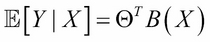
Recall that in linear regression, we assume the following functional form between the dependent variable Y and independent variable X:

Here, is a set of basis functions and is the parameter vector. Usually, it is assumed that , so represents an intercept or a bias term. Also, it is assumed that is a noise term distributed according to the normal distribution with mean zero and variance . We also showed that this results in the following equation:

One can generalize the preceding equation to incorporate not only the normal distribution for noise but any distribution in the exponential family (reference 1 in the References section of this chapter). This is done by defining the following equation:

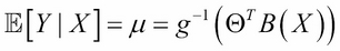
Here, g is called a link function. The well-known models, such as logistic regression, log-linear models, Poisson regression, and so on, are special cases of GLM. For example, in the case of ordinary linear regression, the link function would be . For logistic regression...

The arm package

In this chapter, for the purpose of illustrating Bayesian regression models, we will use the arm package of R. This package was developed by Andrew Gelman and co-workers, and it can be downloaded from the website at http://CRAN.R-project.org/package=arm.

The arm package has the bayesglm function that implements the Bayesian generalized linear model with an independent normal, t, or Cauchy prior distributions, for the model coefficients. We will use this function to build Bayesian regression models.

The Energy efficiency dataset

We will use the Energy efficiency dataset from the UCI Machine Learning repository for the illustration of Bayesian regression (reference 2 in the References section of this chapter). The dataset can be downloaded from the website at http://archive.ics.uci.edu/ml/datasets/Energy+efficiency. The dataset contains the measurements of energy efficiency of buildings with different building parameters. There are two energy efficiency parameters measured: heating load (Y1) and cooling load (Y2).

The building parameters used are: relative compactness (X1), surface area (X2), wall area (X3), roof area (X4), overall height (X5), orientation (X6), glazing area (X7), and glazing area distribution (X8). We will try to predict heating load as a function of all the building parameters using both ordinary regression and Bayesian regression, using the glm functions of the arm package. We will show that, for the same dataset, Bayesian regression gives significantly smaller prediction...

Regression of energy efficiency with building parameters

In this section, we will do a linear regression of the building's energy efficiency measure, heating load (Y1) as a function of the building parameters. It would be useful to do a preliminary descriptive analysis to find which building variables are statistically significant. For this, we will first create bivariate plots of Y1 and all the X variables. We will also compute the Spearman correlation between Y1 and all the X variables. The R script for performing these tasks is as follows:

>library(ggplot2)
>library(gridExtra)

>df <- read.csv("ENB2012_data.csv",header = T)
>df <- df[,c(1:9)]
>str(df)
>df[,6] <- as.numeric(df[,6])
>df[,8] <- as.numeric(df[,8])

>attach(df)
>bp1 <- ggplot(data = df,aes(x = X1,y = Y1)) + geom_point()
>bp2 <- ggplot(data = df,aes(x = X2,y = Y1)) + geom_point()
>bp3 <- ggplot(data = df,aes(x = X3,y = Y1)) + geom_point()
>bp4 <- ggplot(data = df,aes...

Simulation of the posterior distribution

If one wants to find out the posterior of the model parameters, the sim( ) function of the arm package becomes handy. The following R script will simulate the posterior distribution of parameters and produce a set of histograms:

>posterior.bayes <- as.data.frame(coef(sim(fit.bayes)))
>attach(posterior.bayes)

>h1 <- ggplot(data = posterior.bayes,aes(x = X1)) + geom_histogram() + ggtitle("Histogram X1")
>h2 <- ggplot(data = posterior.bayes,aes(x = X2)) + geom_histogram() + ggtitle("Histogram X2")
>h3 <- ggplot(data = posterior.bayes,aes(x = X3)) + geom_histogram() + ggtitle("Histogram X3")
>h4 <- ggplot(data = posterior.bayes,aes(x = X4)) + geom_histogram() + ggtitle("Histogram X4")
>h5 <- ggplot(data = posterior.bayes,aes(x = X5)) + geom_histogram() + ggtitle("Histogram X5")
>h7 <- ggplot(data = posterior.bayes,aes(x = X7)) + geom_histogram() + ggtitle("Histogram X7")
>grid.arrange(h1,h2,h3,h4,h5,h7,nrow...

Exercises

1. Use the multivariate dataset named Auto MPG from the UCI Machine Learning repository (reference 3 in the References section of this chapter). The dataset can be downloaded from the website at https://archive.ics.uci.edu/ml/datasets/Auto+MPG. The dataset describes automobile fuel consumption in miles per gallon (mpg) for cars running in American cities. From the folder containing the datasets, download two files: auto-mpg.data and auto-mpg.names. The auto-mpg.data file contains the data and it is in space-separated format. The auto-mpg.names file has several details about the dataset, including variable names for each column. Build a regression model for the fuel efficiency, as a function displacement (disp), horse power (hp), weight (wt), and acceleration (accel), using both OLS and Bayesian GLM. Predict the values for mpg in the test dataset using both the OLS model and Bayesian GLM model (using the bayesglm function). Find the Root Mean Square Error (RMSE) values for OLS and...

References

1. Friedman J., Hastie T., and Tibshirani R. The Elements of Statistical Learning – Data Mining, Inference, and Prediction. Springer Series in Statistics. 2009

2. Tsanas A. and Xifara A. "Accurate Quantitative Estimation of Energy Performance of Residential Buildings Using Statistical Machine Learning Tools". Energy and Buildings. Vol. 49, pp. 560-567. 2012

3. Quinlan R. "Combining Instance-based and Model-based Learning". In: Tenth International Conference of Machine Learning. 236-243. University of Massachusetts, Amherst. Morgan Kaufmann. 1993. Original dataset is from StatLib library maintained by Carnegie Mellon University.

Summary

In this chapter, we illustrated how Bayesian regression is more useful for prediction with a tighter confidence interval using the Energy efficiency dataset and the bayesglm function of the arm package. We also learned how to simulate the posterior distribution using the sim function in the same R package. In the next chapter, we will learn about Bayesian classification.