Vehicle Detection Using OpenCV and Deep Learning

Object detection is one of the important applications of computer vision used in self-driving cars. Object detection in images means not only identifying the kind of object but also localizing it within the image by generating the coordinates of a bounding box that contains the object. We can summarize object detection as follows:

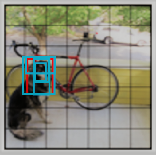
An example of object detection can be seen in the following image:

Fig 11.1: Object detection

Here, you can see that the biker is detected as a person and that the bike is detected as a motorbike. 

In this chapter, we are going to use OpenCV and You Only Look Once (YOLO) as the deep learning architecture for vehicle detection. Due to this, we'll learn about the state-of-the-art image detection algorithm known as YOLO. YOLO can view an image...

What makes YOLO different?

In this chapter, we will be using version 3 of the YOLO object detection algorithm, which further improves upon the old version of YOLO in terms of both speed and accuracy. Let's see how YOLO is different from other object detection networks:

• YOLO looks at the whole image during the testing process, so the prediction of YOLO is informed by the global context of the image.
• In general, networks such as R-CNN require thousands of networks to predict a single image, but in the case of YOLO, only one network is required to look into the image and make predictions.
• Due to the use of a single neural network, YOLO is 1,000x faster than other object detection networks (https://pjreddie.com/darknet/yolo/).
• YOLO treats detection as a regression problem.
• YOLO is extremely fast and accurate.

YOLO works as follows:

1. YOLO takes the input image and divides it into a grid of SxS. Every grid cell predicts one entity.
2. YOLO applies image classification and localization...

The YOLO loss function

The YOLO loss function is calculated in the following steps: 

1. First, we find the bounding boxes with the highest intersection over union (IoU) and with the correct bounding boxes.
2. Then, we calculate the confidence loss, which means the probability of the object being present inside a given bounding box.
3. Next, we calculate the classification loss, which indicates the present class of objects within the bounding box.
4. Finally, we calculate the coordinate loss for matching the detected boxes.

In summary, the total loss function is as follows:

In the next section, we will learn about the YOLO architecture.

The YOLO architecture 

The YOLO architecture is inspired by the image classification model created by GoogLeNet. The YOLO network consists of 24 convolutional layers, followed by two fully connected layers. It also has alternating 1×1 convolutional layers, which reduce the feature spaces from preceding layers. 

The convolution layers that are used in YOLO are from the pre-trained model of the ImageNet task, sampled at half the resolution (244x244), and then double the resolution. YOLO uses leaky ReLU for all the layers and a linear activation function for the final layers.

The following diagram shows the model architecture of YOLO:

Fig 11.2: YOLO architecture

The following is a link to the official YOLO website: https://pjreddie.com/darknet/yolo/.

In the next section, we will learn about the different types of YOLO.

Fast YOLO

Fast YOLO is – as the name suggests – a faster version of YOLO. Fast YOLO uses nine convolutional layers and fewer filters than YOLO. The training and testing parameters are the same in both models. The output of Fast YOLO is 7x7x30 tensors.

YOLO v2

YOLO v2 (also known as YOLO9000) increased YOLO's original input size from 224x224 to 448x448. It was observed that this increase in size resulted in an improved mAP. YOLO v2 also uses batch normalization, which leads to a significant improvement in the accuracy of the model. It also resulted in an improvement in the detection of small objects, which was achieved by dividing the entire image using a 13x13 grid. In order to obtain good priors (anchors) for the model, YOLO v2 runs k-means clustering on the bounding box scale. YOLO v2 also uses five anchor boxes, as shown in the following image:

Fig 11.3: Anchor boxes

In the preceding image, the boxes in blue are anchor boxes, while the box in red is the ground truth box for the object.

YOLOv2 uses the Darknet architecture for object classification and has 19 convolution layers, five max-pooling layers, and a softmax layer.

YOLO v3

YOLO v3 is the most popular model of YOLO. It uses nine anchor boxes. YOLO V3 uses logistic regression for prediction instead of Softmax (which is used in YOLO v2). YOLO v3 also uses the Darknet-53 network for feature extraction, which consists of 53 convolutional layers.

In the next section, we will implement YOLO for object detection in both image and video.

Implementation of YOLO object detection

Now, let's explore how to implement YOLO v3 with Python. We will be using an implementation of YOLO v3 that has been trained on the COCO dataset. 

The COCO dataset contains over 1.5 million object instances within 80 different object categories. We will use a pre-trained model that has been trained on the COCO dataset and explore its capabilities. Realistically, it would take many hours of training, even after using a high-end GPU, to achieve a reasonable model that can predict the required classes with good accuracy. Therefore, we will download the weights of the pre-trained network. This network is hugely complex, and the actual H5 file for the weights is over 200 MB in size. 

Common objects in content (COCO) is a large-scale object detection, segmentation, and captioning dataset. The official website for COCO is http://cocodataset.org/#home.
COCO has several features:

• Object segmentation
• Recognition in context
• Superpixel stuff...

Importing the libraries

The first step is to import the libraries.

We will import the numpy, openCV, and YOLO libraries for implementation purposes:

import os
import time
import cv2
import numpy as np
from model.yolo_model import YOLO

In the next section, we will write code for the image function so that we can resize the image, as per the architecture.

Processing the image function

Next, we will write a process image function. This function will reduce or expand the image, depending on its original size.

Here, we want to transform the image as per the input for the YOLO model:

def process_image(img):
   """Resize, reduce and expand image.

    # Argument:
        img: original image.

    # Returns
        image_org: ndarray(64, 64, 3), processed image.
    """
    image_org = cv2.resize(img, (416, 416),
     interpolation=cv2.INTER_CUBIC)
     image_org = np.array(image_org, dtype='float32')
     image_org /= 255.
     image_org = np.expand_dims(image_org, axis=0)

     return image_org

In the next section, we will write a class function so that we can access the classes from a text file.

The get class function

The class function will help us grab classes from the classes text file. We can find the coco_classes.txt file in the data folder in the project, in the section, Importing YOLO.

The COCO dataset contains almost 80 classes. It can detect them as follows:

def get_classes(file):
    """Get classes name.

    # Argument:
        file: classes name for database.

    # Returns
        class_names: List, classes name.

    """
    with open(file) as f:
     name_of_class = f.readlines()
     name_of_class_names = [c.strip() for c in name_of_class]

     return name_of_class

In the next section, we will write code for the box function, which is useful for drawing boxes around the objects in images.

Draw box function

The draw function will draw a box inside the identified image and put text on the image as a label, as well as place a prediction percentage for the identified class.

We will use OpenCV techniques in this step:

def draw_box(image, image_boxes, image_scores, image_classes, image_all_classes):
    """Draw the boxes on the image.

    # Argument:
        image: original image.
        image_boxes: ndarray, boxes of objects.
        image_classes: ndarray, classes of objects.
        image_scores: ndarray, scores of objects.
        image_all_classes: all classes name.
 """
     for box, score, cl in zip(image_boxes, image_scores, image_classes):
     x, y, w, h = box

     image_top = max(0, np.floor(x + 0.5).astype(int))
     image_left = max(0, np.floor(y + 0.5).astype(int))
     image_right = min(image.shape[1], np.floor(x + w + 0.5).astype(int))
     image_bottom = min(image.shape[0], np.floor(y + h + 0.5).astype(int))

     cv2.rectangle(image, (image_top...

Detect image function

The detect image function takes the image and uses the YOLO3 network to predict the class of objects within the image using yolo.predict. The code for this is as follows:

def detect_image(image, yolo, all_classes):
    """Use yolo v3 to detect images.

    # Argument:
        image: original image.
        yolo: YOLO, yolo model.
        all_classes: all classes name.

    # Returns:
        image: processed image.
    """
    pimage = process_image(image)

    start = time.time()
     image_boxes, image_classes, image_scores = yolo.predict(pimage, image.shape)
     end = time.time()

     print('time: {0:.2f}s'.format(end - start))

     if boxes is not None:
     draw_boxes(image, image_boxes, image_scores, image_classes, image_all_classes)

    return image

In the next section, we will write some code that will detect objects in videos.

Detect video function

If we want to track a person or vehicle in a video, we can use the following function:

def detect_video(video, yolo, all_classes):
    """Use yolo v3 to detect video.

    # Argument:
        video: video file.
        yolo: YOLO, yolo model.
        all_classes: all classes name.
    """
    video_path = os.path.join("videos", "test", video)
    camera = cv2.VideoCapture(video_path)
    cv2.namedWindow("detection", cv2.WINDOW_AUTOSIZE)

    # Prepare for saving the detected video
    sz = (int(camera.get(cv2.CAP_PROP_FRAME_WIDTH)),
        int(camera.get(cv2.CAP_PROP_FRAME_HEIGHT)))
    fourcc = cv2.VideoWriter_fourcc(*'mpeg')

    
    vout = cv2.VideoWriter()
    vout.open(os.path.join("videos", "res", video), fourcc, 20, sz, True)

    while True:
        res, frame = camera.read()

        if not res:
            break

        image = detect_image(frame, yolo, all_classes)
        cv2.imshow("...

Importing YOLO

In this section, we will create an instance of YOLO classes. Note that it may take a little time as the YOLO model needs to load up:

yolo = YOLO(0.6, 0.5)
file = 'data/coco_classes.txt'
all_classes = get_classes(file)

In the next section, we will test the implementation of the YOLO model by predicting objects in an image, as well as a video.

Detecting objects in images

In this section, we will predict the objects present in an image using YOLO. In the following code block we will start with importing the image:

f = 'image.jpg'
path = 'images/'+f
image = cv2.imread(path)

The input image looks as follows:

Fig 11.4: Input image

We will perform the prediction using detect_image method in the following code:

image = detect_image(image, yolo, all_classes)
cv2.imwrite('images/res/' + f, image)

This yields the following prediction:

Fig 11.5: Output image

Here, we can observe that it predicted a person with 100% accuracy and the motorbike with 100% accuracy as well. You can take different images and experiment with this yourself!

Detecting objects in videos

Detecting objects in videos may take time. We will import the video name library.mp4 and perform prediction using detect_video method:

# # detect videos one at a time in videos/test folder 
video = 'library.mp4'
detect_video(video, yolo, all_classes)

This yields the following prediction:

Fig 11.6: Prediction

Here, YOLO predicted a person and a bicycle with 100% confidence!

Summary

In this chapter, we learned about object detection, which is an important aspect of autonomous vehicles. We used a popular pre-trained model called YOLO. Then, we created a software pipeline to perform object predictions on both images and videos and also saw the high quality of YOLO's performance.

This is the last hands-on implementation in this book. In the next chapter, we will read about the next steps to follow in the field of self-driving cars. We will also learn about sensor fusion.