
We will cover the following recipes in this chapter:
- Computing ordinary least squares estimates
- Reporting results with the sjPlot package
- Finding correlation between the features
- Testing hypothesis
- Testing homoscedasticity
- Implementing sandwich estimators
- Variable selection
- Ridge regression
- Working with LASSO
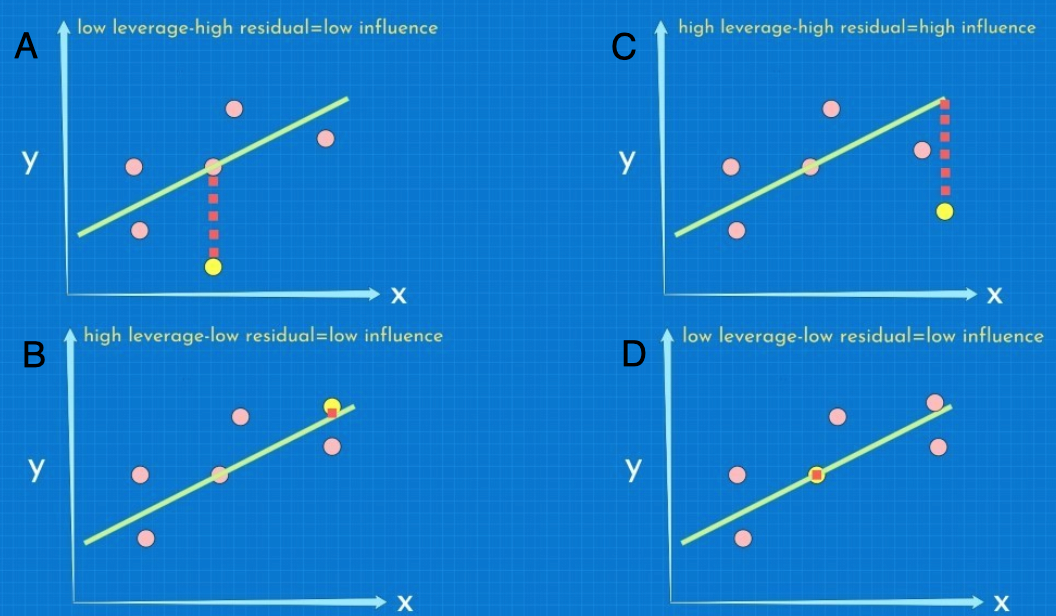
- Leverage, residuals, and influence

 . It should be noted that we need to compute an inverse, and that can only be done if the determinant is different from zero. The determinant will be zero if there is a linear dependency between the variables.
  where
where  is the estimated residual standard error.
  estimates using both the