


Making an app from scratch
Now that we’ve tried out the apps others have made, let’s make our own! This app is going to focus on using the central limit theorem, which is a fundamental theorem of statistics that says that if we randomly sample with replacement enough from any distribution, then the distribution of the mean of our samples will approximate the normal distribution.
We are not going to prove this with our app, but instead, let’s try to generate a few graphs that help explain the power of the central limit theorem. First, let’s make sure that we’re in the correct directory (in this case, the streamlit_apps folder that we created earlier), make a new folder called clt_app, and toss in a new file.
The following code makes a new folder called clt_app, and again creates an empty Python file, this time called clt_demo.py:
mkdir clt_app
cd clt_app
touch clt_demo.py
Whenever we start a new Streamlit app, we want to make sure to import Streamlit (often aliased in this book and elsewhere as st). Streamlit has unique functions for each type of content (text, graphs, pictures, and other media) that we can use as building blocks for all of our apps. The first one we’ll use is st.write(), which is a function that takes a string (and as we’ll see later, almost any Pythonic object, such as a dictionary) and writes it directly into our web app in the order that it is called. As we are calling a Python script, Streamlit sequentially looks through the file and, every time it sees one of the functions, designates a sequential slot for that piece of content. This makes it very easy to use, as you can write all the Python you’d like, and when you want something to appear on the app you’ve made, you can simply use st.write() and you’re all set.
In our clt_demo.py file, we can start with the basic 'Hello World' output using st.write(), using the following code:
import streamlit as st
st.write('Hello World')
Now we can test this by running the following code in the terminal:
streamlit run clt_demo.py
We should see the string 'Hello World' printed on our app, so all is good so far. The following figure is a screenshot of our app in Safari:
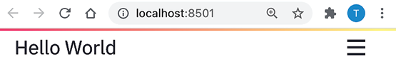
Figure 1.2: Hello World app
There are three items to note in this screenshot. First, we see the string as we wrote it, which is great. Next, we see that the URL points to localhost:8501, which is just telling us that we’re hosting this locally (that is, it’s not on the internet anywhere) through port 8501. We don’t need to understand almost anything about the port system on computers, or the Transmission Control Protocol (TCP). The important thing here is that this app is local to your computer. Later in this book, we’ll learn how to take the local apps we create and share them with anyone via a link! The third important item to note is the hamburger icon at the top right. The following screenshot shows us what happens when we click the icon:
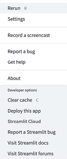
Figure 1.3: Icon options
This is the default options panel for Streamlit apps. Throughout this book, we’ll discuss each of these options in depth, especially the non-self-explanatory ones such as Clear cache. All we have to know for now is that if we want to rerun the app or find settings or the documentation, we can use this icon to find almost whatever we need.
When we host applications so that others can use them, they’ll see this same icon but have some different options (for example, users will not be able to clear the cache). We’ll discuss this in greater detail later as well. Now back to our central limit theorem app!
The next step is going to be generating a distribution that we want to sample from with replacement. I’m choosing the binomial here. We can read the following code as simulating 1,000 coin flips using the Python package NumPy, and printing out the mean number of heads from those 1,000 coin flips:
import streamlit as st
import numpy as np
binom_dist = np.random.binomial(1, .5, 100)
st.write(np.mean(binom_dist))
Now, given what we know about the central limit theorem, we would expect that if we sampled from binom_dist enough times, the mean of those samples would approximate the normal distribution.
We’ve already discussed the st.write() function. Our next foray into writing content to the Streamlit app is through graphs. st.pyplot() is a function that lets us use all the power of the popular matplotlib library and push our matplotlib graph to Streamlit. Once we create a figure in matplotlib, we can explicitly tell Streamlit to write that to our app with the st.pyplot() function. So, all together now! This app simulates 1,000 coin flips and stores those values in a list we call binom_dist. We then sample (with replacement) 100 from that list, take the mean, and store that mean in the cleverly named variable list_of_means. We do that 1,000 times (which is overkill – we could do this even with dozens of samples), and then plot the histogram. After we do this, the result of the following code should show a bell-shaped distribution:
import streamlit as st
import numpy as np
import matplotlib.pyplot as plt
binom_dist = np.random.binomial(1, .5, 1000)
list_of_means = []
for i in range(0, 1000):
     list_of_means.append(np.random.choice(binom_dist, 100, replace=True).mean())
fig, ax = plt.subplots()
ax = plt.hist(list_of_means)
st.pyplot(fig)
Each run of this app will create a new bell curve. When I ran it, my bell curve looked like the following figure. If your graph isn’t exactly what you see in the next figure (but is still a bell!), that’s totally fine because of the random sampling used in our code:
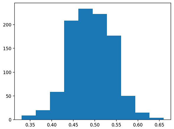
Figure 1.4: Bell curve
As you probably noticed, we first created an empty figure and empty axes for that figure by calling plt.subplots(), and then assigned the histogram we created to the ax variable. Because of this, we were able to explicitly tell Streamlit to show the figure in our Streamlit app.
This is an important step, as in Streamlit versions, we can also skip this step, not assign our histogram to any variable, and then call st.pyplot() directly afterward. The following code takes this approach:
import streamlit as st
import numpy as np
import matplotlib.pyplot as plt
binom_dist = np.random.binomial(1, .5, 1000)
list_of_means = []
for i in range(0, 1000):
     list_of_means.append(np.random.choice(binom_dist, 100, replace=True).mean())
plt.hist(list_of_means)
st.pyplot()
I don’t recommend this method, as it can give you some unexpected results. Take this example, where we want to first make our histogram of means, and then make another histogram of a new list filled only with the number 1.
Take a second and guess what the following code would do. How many graphs would we get? What would the output be?
import streamlit as st
import numpy as np
import matplotlib.pyplot as plt
binom_dist = np.random.binomial(1, .5, 1000)
list_of_means = []
for i in range(0, 1000):
     list_of_means.append(np.random.choice(binom_dist, 100, replace=True).mean())
plt.hist(list_of_means)
st.pyplot()
plt.hist([1,1,1,1])
st.pyplot()
I would expect this to show two histograms, the first one of list_of_means, and the second one of the lists of 1s:
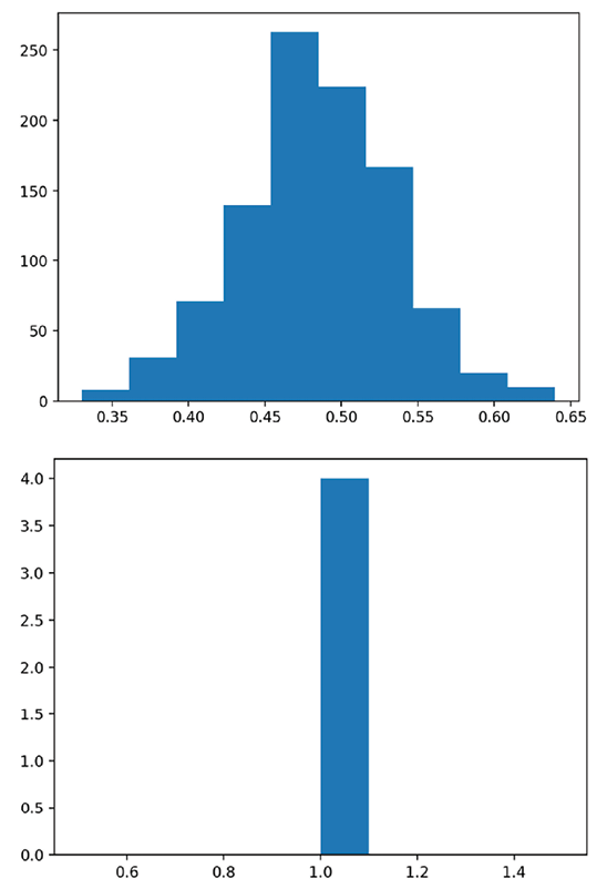
Figure 1.5: A tale of two histograms
What we actually get is different! The second histogram has data from the first and the second list! When we call plt.hist() without assigning the output to anything, matplotlib tacks the new histogram onto the old graph, which is stored globally, and Streamlit pushes that new one to our app. You may also get a PyplotGlobalUseWarning when you run the preceding code, depending on your matplotlib version. Don’t worry, we will fix this in the next section!
Here’s a solution to this issue. If we instead explicitly created two graphs, we could call the st.pyplot() function wherever we liked after the graph was generated, and have greater control over where exactly our graphs were placed. The following code separates the two graphs explicitly:
import streamlit as st
import numpy as np
import matplotlib.pyplot as plt
binom_dist = np.random.binomial(1, .5, 1000)
list_of_means = []
for i in range(0, 1000):
     list_of_means.append(np.random.choice(binom_dist, 100, replace=True).mean())
fig1, ax1 = plt.subplots()
ax1 = plt.hist(list_of_means)
st.pyplot(fig1)
fig2, ax2 = plt.subplots()
ax2 = plt.hist([1,1,1,1])
st.pyplot(fig2)
The preceding code plots both histograms separately by first defining separate variables for each figure and axis using plt.subplots() and then assigning the histogram to the appropriate axis. After this, we can call st.pyplot() using the created figure, which produces the following app:
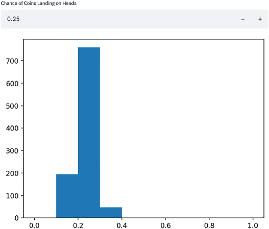
Figure 1.6: Fixed histograms
We can clearly see in the preceding figure that the two histograms are now separated, which is the desired behavior. We will very often plot multiple visualizations in Streamlit and will use this method for the rest of the book.
Matplotlib is an extremely popular library for data visualization but has some serious flaws when used within data apps. It is not interactive by default, it is not particularly pretty, and it also can slow down very large apps. Later in this book, we’ll switch over to more performant and interactive libraries.
Now, on to accepting user input!
Using user input in Streamlit apps
As of now, our app is just a fancy way to show our visualizations. But most web apps take some user input or are dynamic, not static visualizations. Luckily for us, Streamlit has many functions for accepting inputs from users, all differentiated by the object that we want to input. There are freeform text inputs with st.text_input(); radio buttons, st.radio(); numeric inputs with st.number_input(); and a dozen more that are extremely helpful for making Streamlit apps. We will explore most of them in detail throughout this book, but we’ll start with numeric input.
From the previous example, we assumed that the coins we were flipping were fair coins and had a 50/50 chance of being heads or tails. Let’s let the user decide what the percentage chance of heads is, assign that to a variable, and use that as an input in our binomial distribution. The number input function takes a label, a minimum and maximum value, and a default value, which I have filled in the following code:
import streamlit as st
import numpy as np
import matplotlib.pyplot as plt
perc_heads = st.number_input(label = 'Chance of Coins Landing on Heads', min_value = 0.0, max_value = 1.0, value = .5)
binom_dist = np.random.binomial(1, perc_heads, 1000)
list_of_means = []
for i in range(0, 1000):
     list_of_means.append(np.random.choice(binom_dist, 100, replace=True).mean())
fig, ax = plt.subplots()
ax = plt.hist(list_of_means, range=[0,1])
st.pyplot(fig)
The preceding code uses the st.number_input() function to collect our percentage, assigns the user input to a variable (perc_heads), then uses that variable to change the inputs to the binomial distribution function that we used before. It also sets our histogram’s x axis to always be between 0 and 1, so we can better notice changes as our input changes. Try and play around with this app for a bit; change the number input and notice how the app responds whenever a user input is changed. For example, here is a result from when we set the numeric input to .25:
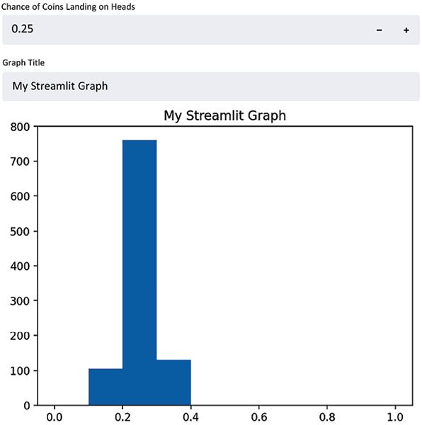
Figure 1.7: An example of a result from when we set the numeric input to .25
As you probably noticed, every time that we changed the input of our script, Streamlit re-ran the entire application. This is the default behavior and is very important to understanding Streamlit performance; we will explore a few ways that allow us to change this default later in the book, such as adding caching or forms! We can also accept text input in Streamlit using the st.text_input() function, just as we did with the numeric input. The next bit of code takes a text input and assigns it to the title of our graph:
import streamlit as st
import numpy as np
import matplotlib.pyplot as plt
perc_heads = st.number_input(label='Chance of Coins Landing on Heads', min_value=0.0,  max_value=1.0, value=.5)
graph_title = st.text_input(label='Graph Title')
binom_dist = np.random.binomial(1, perc_heads, 1000)
list_of_means = []
for i in range(0, 1000):
list_of_means.append(np.random.choice(binom_dist, 100, replace=True).mean())
fig, ax = plt.subplots()
plt.hist(list_of_means, range=[0,1])
plt.title(graph_title)
st.pyplot(fig)
This creates a Streamlit app with two inputs, both a numeric input and a text input, and uses them both to change our Streamlit app. Finally, this results in a Streamlit app that looks like the next figure, with dynamic titles and probabilities:
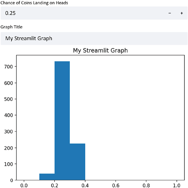
Figure 1.8: A Streamlit app with dynamic titles and probabilities
Now that we have worked a bit with user input, let’s talk about text and Streamlit apps more deeply.