Chapter 3. Jupyter R Scripting

Jupyter's native language is Python. Once Jupyter (essentially, IPython before being renamed) became popular for data analysis, a number of people were interested in using the suite of R programming analysis tools that are available in a Jupyter Notebook.

In this chapter, we will cover the following topics:

• Adding R scripting to your installation

• Basic R scripting

• R dataset access (from a library)

• R graphics

• R cluster analysis

• R forecasting

Adding R scripting to your installation

Two big installation platforms are Mac and Windows. There are separate, but similar, steps required to make R scripting available in your Jupyter installation.

Adding R scripts to Jupyter on a Mac

If you are operating a Mac, you can add R scripting using the command-line:

conda install -c r r-essentials

This will start off with a large installation of the R environment, which contains a number of common packages:

bos-mpdc7:~ dtoomey$ conda install -c r r-essentials
Fetching package metadata: ......
Solving package specifications: .........
Package plan for installation in environment /Users/dtoomey/miniconda3:
    The following packages will be downloaded:
    package                    |            build
    ---------------------------|-----------------
    jbig-2.1                   |                0          31 KB
    jpeg-8d                    |                2         210 KB
    libgcc-4.8.5               |                1         785 KB...

Basic R in Jupyter

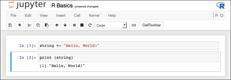
Start a new R notebook and call it R Basics. We can enter a small script just so we can see how the steps progress for an R script. Enter the following into separate cells of your notebook:

myString <- "Hello, World!"
print (myString)

You will end up with a starting screen that looks like this:

We should note the aspects of the R notebook view:

• We have the R logo in the upper-right corner. You will see this logo running in other R installations.

• There is also the peculiar R O just below the R icon. The unfilled circle indicates that the kernel is at rest, and the filled circle indicates the kernel is working.

• The rest of the menu items are the same as we have seen before.

This is a very simple script-set a variable in one cell then print out its value in another cell. Once executed (Cell | Run All), you will see your results:

So, just as if you ran the script in an R interpreter, you get your output (with the numerical prefix). Jupyter has counted the statements so we...

R dataset access

For this example, we will use the Iris dataset. Iris is built into R installations and is available directly. Let's just pull in the data, gather some simple statistics, and plot the data. This will show R accessing a dataset in Jupyter, using an R built-in package, as well as some available statistics (since we have R), and the interaction with R graphics.

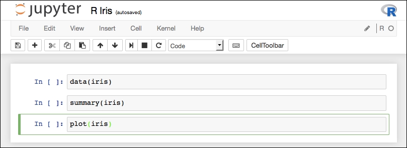
The script we will use is as follows:

dataset(iris)
summary(iris)
plot(iris)

If we enter this small script into a new R notebook, we get an initial display that looks like the following:

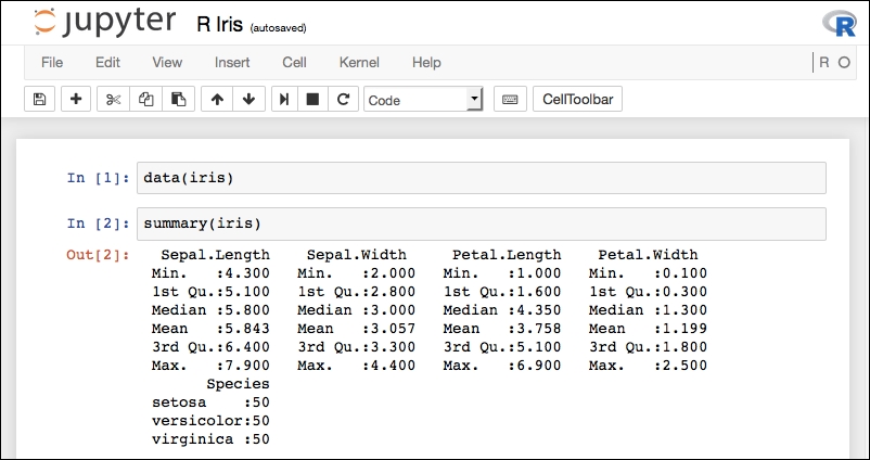
I would expect the standard R statistical summary as output, and I know the Iris plot is pretty interesting. We can see exactly what happened in the following screenshot:

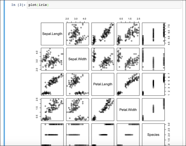
The plot continues in the following screenshot as it wouldn't fit into a single screenshot:

R visualizations in Jupyter

A common use of R is to use several visualizations, which are available depending on the underlying data. In this section, we will go over some of them to see how R interacts with Jupyter.

R 3D graphics in Jupyter

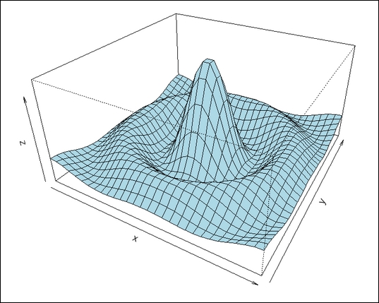
One of the packages available for 3D graphics is persp. The persp package draws perspective plots over a 2D space.

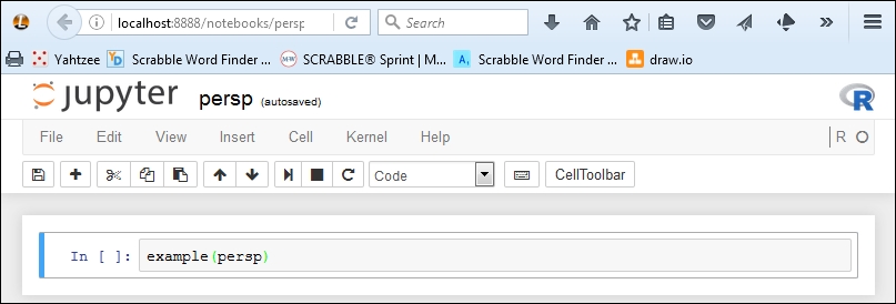
We can enter a basic persp command in a new notebook and have something like this:

Once we run the step (Cell | Run All), we can see the display in the following screenshot. The first part is the script involved to generate the graphic (this is part of the example code):

Then we see the following graphic display:

R 3D scatterplot in Jupyter

The R lattice package has a cloud function that will produce 3D scatterplots.

The script we will use is as follows:

# make sure lattice package is installed
install.package("lattice")
# in a standalone R script you would have a command to download the lattice library - this is not needed in Jupyter
library...

R cluster analysis

In this example, we use R's cluster analysis functions to determine the clustering in the wheat dataset from http://www.ics.uci.edu/.

The R script we want to use in Jupyter is the following:

# load the wheat data set from uci.edu
wheat <- read.csv("http://archive.ics.uci.edu/ml/machine-learning-databases/00236/seeds_dataset.txt", sep="\t")
# define useful column names
colnames(wheat) <-c("area", "perimeter", "compactness", "length", "width", "asymmetry", "groove", "undefined")
# exclude incomplete cases from the data
wheat <- wheat[complete.cases(wheat),]
# calculate the clusters
fit <- kmeans(wheat, 5)
fit

Once entered into a notebook, we have something like this:

The resulting generated cluster information is K-means clustering with five clusters of sizes 29, 57, 65, 15, and 32. (Note that, since I had not set the seed value for random number to use, your results may vary.)

Cluster means are:

      area perimeter compactness   length    width asymmetry  ...

R forecasting

For this example, we will forecast the Fraser River levels given the data from  https://datamarket.com/data/set/22nm/fraser-river-at-hope-1913-1990#!ds=22nm&display=line . I was not able to find a suitable source so I extracted the data by hand from the site into a local file.

We will be using the R forecast package. You have to add this package to your setup (as described at the start of this chapter).

The R script we will be using is as follows:

library(forecast)
fraser <- scan("fraser.txt")
plot(fraser)
fraser.ts <- ts(fraser, frequency=12, start=c(1913,3))
fraser.stl = stl(fraser.ts, s.window="periodic")
monthplot(fraser.stl)
seasonplot(fraser.ts)

The output of interest in this example are the three plots: simple plot, monthly, and computed seasonal.

The simple plot (using the R plot command) is like the following screenshot. There is no apparent organization or structure:

The monthly plot (using the monthplot command) is like the following screenshot. River flows...

Summary

In this chapter, we added the ability to use R scripts in your Jupyter Notebook. We added an R library not included in the standard R installation and we made a Hello World script in R. We then saw R data access built-in libraries and some of the simpler graphics and statistics that are automatically generated. We used an R script to generate 3D graphics in a couple of different ways. We then performed a standard cluster analysis (which I think is one of the basic uses of R) and used one of the available forecasting tools.

In the next chapter, we will learn all about Julia scripting in a Jupyter Notebook.