


The anatomy of a standard ML workflow
In a traditional ML application, professionals have to train a model using a set of input data. If this data is not in the proper form, an expert may have to apply some data preprocessing techniques, such as feature extraction, feature engineering, or feature selection.
Once the data is ready and the model can be trained, the next step is to select the right algorithm and optimize the hyperparameters to maximize the accuracy of the model's predictions. Each step involves time-consuming challenges, and typically also requires a data scientist with the experience and knowledge to be successful. In the following figure, we can see the main steps represented in a typical ML pipeline:
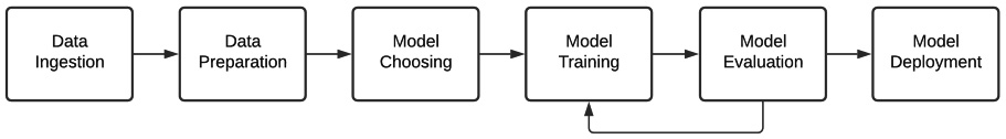
Figure 1.1 – ML pipeline steps
Each of these pipeline processes involves a series of steps. In the following sections, we describe each process and related concepts in more detail.
Data ingestion
Piping incoming data to a data store is the first step in any ML workflow. The target here is to store that raw data without doing any transformation, to allow us to have an immutable record of the original dataset. The data can be obtained from various data sources, such as databases, message buses, streams, and so on.
Data preprocessing
The second phase, data preprocessing, is one of the most time-consuming tasks in the pipeline and involves many sub-tasks, such as data cleaning, feature extraction, feature selection, feature engineering, and data segregation. Let's take a closer look at each one:
- The data cleaning process is responsible for detecting and fixing (or deleting) corrupt or wrong records from a dataset. Because the data is unprocessed and unstructured, it is rarely in the correct form to be processed; it implies filling in missing fields, removing duplicate rows, or normalizing and fixing other errors in the data.
- Feature extraction is a procedure for reducing the number of resources required in a large dataset by creating new features from the combination of others (and eliminating the original ones). The main problem when analyzing large datasets is the number of variables to take into account. Processing a large number of variables generally requires a lot of hardware resources, such as memory and computing power, and can also cause overfitting, which means that the algorithm works very well for training samples and generalizes poorly for new samples. Feature extraction is based on the construction of new variables, combining existing ones to solve these problems without losing precision in the data.
- Feature selection is the process of selecting a subset of variables to use in building the model. Performing feature selection simplifies the model (making it more interpretable for humans), reduces training times, and improves generalization by reducing overfitting. The main reason to apply feature selection methods is that the data contains some features that can be redundant or irrelevant, so removing them wouldn't incur much loss of information.
- Feature engineering is the process by which, through data mining techniques, features are extracted from raw data using domain knowledge. This typically requires a knowledgeable expert and is used to improve the performance of ML algorithms.
Data segregation consists of dividing the dataset into two subsets: a train dataset for training the model and a test dataset for testing the prediction modeling.
Modeling is divided into three parts:
- Choose candidate models to evaluate.
- Train the chosen model (improve it).
- Evaluate the model (compare it with others).
This process is iterative and involves testing various models until one is obtained that solves the problem in an efficient way. The following figure shows a detailed schema of the modeling phases of the ML pipeline:
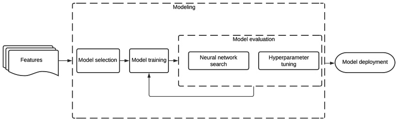
Figure 1.2 – Modeling phases of the ML pipeline
After taking an overview of the modeling phase, let's look at each modeling step in more detail.
Let's dive deeper into the three parts of modeling to have a detailed understanding of them.
Model selection
In choosing a candidate model to use, in addition to performance, it is important to consider several factors, such as readability (by humans), ease of debugging, the amount of data available, as well as hardware limitations for training and prediction.
The main points to take into account for selecting a model would be as follows:
- Interpretability and ease of debugging: How to know why a model made a specific decision. How do we fix the errors?
- Dataset type: There are algorithms that are more suitable for specific types of data.
- Dataset size: How much data is available and will this change in the future?
- Resources: How much time and resources do you have for training and prediction?
Model training
This process uses the training dataset to feed each chosen candidate model, allowing the models to learn from it by applying a backpropagation algorithm that extracts the patterns found in the training samples.
The model is fed with the output data from the data preprocessing step. This dataset is sent to the chosen model and once trained, both the model configuration and the learned parameters will be used in the model evaluation.
Model evaluation
This step is responsible for evaluating model performance using test datasets to measure the accuracy of the prediction. This process involves tuning and improving the model, generating a new candidate model version to be trained again.
Model tuning
This model evaluation step involves modifying hyperparameters such as the learning rate, the optimization algorithm, or model-specific architecture parameters, such as the number of layers and types of operations for neural networks. In standard ML, these procedures need to be performed manually by an expert.
Other times, the evaluated model is discarded, and another new model is chosen for training. Often, starting with a previously trained model through transfer learning leads to shortened training time as well as better precision on the final model predictions.
Since the main bottleneck is the training time, the adjustment of the models should focus on efficiency and reproducibility so that the training is as fast as possible and someone can reproduce the steps that have been taken to improve performance.
Model deployment
Once the best model is chosen, it is usually put into production through an API service to be consumed by the end user or other internal services.
Usually, the best model is selected to be deployed in one of two deployment modes:
- Offline (asynchronous): In this case, the model predictions are calculated in a batch process periodically and stored in a data warehouse as a key-value database.
- Online (synchronous): In this mode, the predictions are calculated in real time.
Deployment consists of exposing your model to a real-world application. This application can be anything, from recommending videos to users of a streaming platform to predicting the weather on a mobile application.
Releasing an ML model into production is a complex process that generally involves multiple technologies (version control, containerization, caching, hot swapping, a/b testing, and so on) and is outside the scope of this book.
Model monitoring
Once in production, the model is monitored to see how it performs in the real world and calibrated accordingly. This schema represents the continuous model cycle, from data ingestion to deployment:
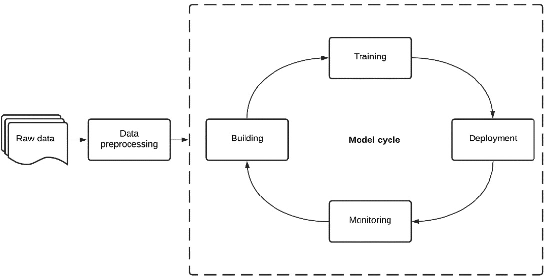
Figure 1.3 – Model cycle phases
In the following sections, we will explain the main reasons why it's really important to monitor your production model.
Why monitor your model?
Your model predictions will degrade over time. This phenomenon is called drift. Drift is a consequence of input data changes, so over time, the predictions get worse in a natural way.
Let's look at the users of a search engine as an example. A predictive model can use user features such as your personal information, search types, and clicked results to predict which ads to show. But after a while, these searches may not represent current user behavior.
A possible solution would be to retrain the model with the most recent data, but this is not always possible and sometimes may even be counterproductive. Imagine training the model with searches at the start of the COVID-19 pandemic. This would only show ads for products related to the pandemic, causing a sharp decline in the number of sales for the rest of the products.
A smarter alternative to combat drift is to monitor our model, and by knowing what is happening, we can decide when and how to retrain it.
How can you monitor your model?
In cases where you have the actual values to compare to the prediction in no time—I mean you have the true labels right after making a prediction—you just need to monitor the performance measures such as accuracy, F1 score, and so on. But often, there is a delay between the prediction and the basic truth; for example, in predicting spam in emails, users can report that an email is spam up to several months after it was created. In this case, you must use other measurement methods based on statistical approaches.
For other complex processes, sometimes it is easier to do traffic/case splitting and monitor pure business metrics, in a case where it is difficult to consider direct relationships between classical ML evaluation metrics and real-world-related instances.
What should you monitor in your model?
Any ML pipeline involves performance data monitoring. Some possible variables of the model to monitor are as follows:
- Chosen model: What kind of model was chosen, and what are the architecture type, the optimizer algorithm, and the hyperparameter values?
- Input data distribution: By comparing the distribution of the training data with the distribution of the input data, we can detect whether the data used for the training represents what is happening now in the real world.
- Deployment date: Date of the release of the model.
- Features used: Variables used as input for the model. Sometimes there are relevant features in production that we are not using in our model.
- Expected versus observed: A scatter plot comparing expected and observed values is often the most widely used approach.
- Times published: The number of times a model was published, represented usually using model version numbers.
- Time running: How long has it been since the model was deployed?
Now that we have seen the different components of the pipeline, we are ready to introduce the main AutoML concepts in the next section.