


Hypothesis Tests
Hypothesis testing is a branch of inferential statistics, that is, a part of the statistics field in which a general conclusion can be done about a large group (a population) based on the analysis and measurements performed on a smaller group (a sample). A typical example could be making an estimation of the average height of a country's citizens (in this case, the population) based on measurements performed on a thousand people (the sample). Hypothesis testing tries to address the question, "Is a certain hypothetical value in line with the value obtained by direct measurements or not?"
Although various statistical tests are known in the literature and in practice, the general idea can be summarized in the following steps:
- Definition of null and alternative hypotheses: In this first step, a null hypothesis (denoted as H0) is defined (let's say H0 is 'the average country's population height is 175 cm'). This is the hypothesis that is going to be tested by the statistical test. The alternative hypothesis (denoted as Ha) consists of the complement statement of the null hypothesis (in our example, the alternative hypothesis, Ha, is 'the average height is not 175 cm'). The null and alternative hypotheses always complement one another.
- Identifying the appropriate test statistic: A test statistic is a quantity whose calculation is based on the sample, and whose value is the basis for accepting or rejecting the null hypothesis. In most of these cases, it can be computed by the following formula:

Figure 1.9: The formula for the test statistic
Here, the sample statistic is the statistic value computed on the sample (in our case, the average height of a thousand people); the value under null hypothesis is the value, assuming that the null hypothesis holds (in this case, 175 cm); and the standard error of the sample statistic is the standard error in the measurement of the sample. Once the test statistic is identified and computed, we have to decide what type of probability distribution it follows. In most of the cases, the following probability distributions will be used: Student's t-distribution (for t-tests); Standard normal or z-distribution (for z-tests); Chi-squared distribution (for a chi-squared test) and F-distribution (for F-tests).
Note
Because exploring probability distributions in more detail is beyond the scope of this book, we refer the reader to the excellent book by Charles Grinstead and Laurie Snell, Introduction to Probability. Take a look at the following link: https://math.dartmouth.edu/~prob/prob/prob.pdf.
Choosing which distribution to use depends on the sample size and the type of test. As a rule of thumb, if the sample size is greater than 30, we can expect that the assumptions of the central limit theorem hold and that the test statistic follows a normal distribution (hence, use a z-test). For a more conservative approach, or for samples with less than 30 entries, a t-test should be used (with a test statistic following Student's t-distribution).
- Specifying the significance level: Once the test statistic has been calculated, we have to decide whether we can reject the null hypothesis or not. In order to do that, we specify a significance level, which is the probability of rejecting a true null hypothesis. A general approach is to specify a level of significance of 5%. This means that we accept that there is a 5% probability that we reject the null hypothesis while being true (for a more conservative approach, we could always use 1% or even 0.5%). Once a significance level is specified, we have to compute the rejection points, which are the values with which the test statistic is compared. If it is larger than the specified rejection point(s), we can reject the null hypothesis and assume that the alternative hypothesis is true. We can distinguish two separate cases here.
- Two-sided tests: These are tests in which the null hypothesis assumes that the value "is equal to" a predefined value. For example, the average height of the population is equal to 175 cm. In this case, if we specify a significance level of 5%, then we have two critical values (one positive and one negative), with the probability of the two tails summing up to 5%. In order to compute the critical values, we have to find the two percentiles of a normal distribution, such that the probability within those two values is equal to 1 minus the significance level. For example, if we assume that the sample mean of the height follows a normal distribution, with a level of significance for our test of 5%, then we need to find the two percentiles, with the probability that a value drawn from a normal distribution falls outside of those values, equal to 0.05. As the probability is split between the two tails, the percentiles that we are looking at are the 2.5 and 97.5 percentiles, corresponding to the values -1.96 and 1.96 for a normal distribution. Hence, we will not reject the null hypothesis if the following holds true:

Figure 1.10: Test statistic limit for a two-sided test
If the preceding formula does not hold true, that is, the test statistic is greater than 1.96 or less than -1.96, we will reject the null hypothesis.
- One-sided tests: These are tests in which the null hypothesis assumes that the value is "greater than" or "less than" a predefined value (for example, the average height is greater than 175 cm). In that case, if we specify a significance level of 5%, we will have only one critical value, with a probability at the tail equal to 5%. In order to find the critical value, we have to find the percentile of a normal distribution, corresponding to a probability of
0.05at the tail. For tests of the "greater than" type, the critical value will correspond to the 5-th percentile, or-1.645(for tests following a normal distribution), while for tests of the "less than" type, the critical value will correspond to the 95-th percentile, or 1.645. In this way, we will reject the null hypothesis for tests "greater than" if the following holds true:
Figure 1.11: Test statistic limit for a one-sided test
Whereas, for tests of the "less than" type, we reject the null hypothesis if the following is the case:

Figure 1.12: Test statistic limit for a one-sided test
Note that, quite often, instead of computing the critical values of a certain significance level, we refer to the p-value of the test. The p-value is the smallest level of significance at which the null hypothesis can be rejected. The p-value also provides the probability of obtaining the observed sample statistic, assuming that the null hypothesis is correct. If the obtained p-value is less than the specified significance level, we can reject the null hypothesis, hence the p-value approach is, in practice, an alternative (and, most of the time, a more convenient) way to perform hypothesis testing.
Let's now provide a practical example of performing hypothesis testing with Python.
Exercise 1.03: Estimating Average Registered Rides
In this exercise, we will show how to perform hypothesis testing on our bike sharing dataset. This exercise is a continuation of Exercise 1.02, Analyzing Seasonal Impact on Rides:
- Start with computing the average number of registered rides per hour. Note that this value will serve in formulating the null hypothesis because, here, you are explicitly computing the population statistic—that is, the average number of rides. In most of the cases, such quantities are not directly observable and, in general, you only have an estimation for the population statistics:
# compute population mean of registered rides
population_mean = preprocessed_data.registered.mean()
- Suppose now that you perform certain measurements, trying to estimate the true average number of rides performed by registered users. For example, register all the rides during the summer of 2011 (this is going to be your sample):
# get sample of the data (summer 2011)
sample = preprocessed_data[(preprocessed_data.season \
                            == "summer") \
                            & (preprocessed_data.yr \
                            == 2011)].registered
- Specify the significance level. A standard value is 0.05 (that is, when performing the statistical test), if the p-value obtained by the statistical test is less than 0.05, you can reject the null hypothesis by at least 95%. The following code snippet shows you how to do that:
# perform t-test and compute p-value
from scipy.stats import ttest_1samp
test_result = ttest_1samp(sample, population_mean)
print(f"Test statistic: {test_result[0]}, \
p-value: {test_result[1]}")
The output should be as follows:
Test statistic: -3.492, p-value: 0.000
The result of the previous test returns a p-value smaller than 0.001, which is less than the predefined critical value. Therefore, you can reject the null hypothesis and assume that the alternative hypothesis is correct.
Note that you have to make an important observation here: You computed the average number of rides on the true population; therefore, the value computed by the statistical test should be the same. So why have you rejected the null hypothesis? The answer to that question lies in the fact that your sample is not a true representation of the population, but rather a biased one. In fact, you selected only entries from the summer of 2011. Therefore, neither data from the full year is present, nor entries from 2012.
- In order to show how such mistakes can compromise the results of statistical tests, perform the test again, but this time taking as a sample 5% of the registered rides (selected randomly). The following code snippet performs that:
# get sample as 5% of the full data
import random
random.seed(111)
sample_unbiased = preprocessed_data.registered.sample(frac=0.05)
test_result_unbiased = ttest_1samp(sample_unbiased, \
                                   population_mean)
print(f"Unbiased test statistic: {test_result_unbiased[0]}, \
p-value: {test_result_unbiased[1]}")
The output should be as follows:
Unbiased test statistic: -2.008, p-value: 0.045
This time, the computed p-value is equal to 0.45, which is much larger than the critical 0.05, and so, you cannot reject the null hypothesis.
Note
To access the source code for this specific section, please refer to https://packt.live/2N3W1la.
You can also run this example online at https://packt.live/3fxDYjt. You must execute the entire Notebook in order to get the desired result.
In this exercise, we performed hypothesis testing with Python on the bike sharing dataset. Furthermore, we saw the importance of having an unbiased sample of the data, as test results can be easily compromised if working with biased data.
Quite often, when performing statistical tests, we want to compare certain statistics on two different groups (for example, the average height between women and men) and estimate whether there is a statistically significant difference between the values obtained in the two groups. Let's denote, with μ1 and μ2, the hypothetical means of the two groups, where we will have:
- A null hypothesis:
H0:μ1-μ2≠ 0 - An alternative hypothesis:
Ha:μ1-μ2≠ 0
Let's denote, with  and
and  , the sample means (that is, the means obtained from the two groups), where the test statistic takes the following form:

Figure 1.13: Test statistic with the sample means
Here, n1 and n2 are the number of samples in the two groups, while  is the pooled estimator of the common variance, computed as follows:

Figure 1.14: Pooled estimator of the common variance
Here,  and
and  are the variances of the two groups. Note that the test statistic, in this case, follows Student's t-distribution with
 n1+n2-2 degrees of freedom.
As in the previous case, most of the time, we don't have to compute the test statistics by ourselves, as Python already provides handy functions for that, plus the alternative approach of accepting or rejecting the null hypothesis using the p-value is still valid.
Let's now focus on a practical example of how to perform a statistical test between two different groups. In the previous section, we observed, graphically, that registered users tend to perform more rides during working days than the weekend. In order to assess this statement, we will perform a hypothesis test in which we will test whether the mean of registered rides during working days is the same as during the weekend. This is done in the following exercise.
Exercise 1.04: Hypothesis Testing on Registered Rides
In this exercise, we will be performing a hypothesis on registered rides. This exercise is a continuation of Exercise 1.03, Estimating Average Registered Rides:
- First, formulate the null hypothesis. As mentioned earlier, you are interested in identifying whether there is a statistically significant difference between registered rides during working days and the weekend. Therefore, our null hypothesis is that the average number of rides for registered users during working days is the same as the average number of rides during the weekend. In other words:
H_0: average registered rides over weekdays-average registered rides over weekend=0and
H_a: average registered rides over weekdays-average registered rides over weekend≠0 - Once the null hypothesis is established, collect data for the two groups. This is done with the following code snippet:
# define mask, indicating if the day is weekend or work day
weekend_days = ['Saturday', 'Sunday']
weekend_mask = preprocessed_data.weekday.isin(weekend_days)
workingdays_mask = ~preprocessed_data.weekday.isin(weekend_days)
# select registered rides for the weekend and working days
weekend_data = preprocessed_data.registered[weekend_mask]
workingdays_data = preprocessed_data.registered[workingdays_mask]
- Perform the two-sample t-tests by using the
scipy.stats.ttest_indfunction:# perform ttest from scipy.stats import ttest_ind test_res = ttest_ind(weekend_data, workingdays_data) print(f"Statistic value: {test_res[0]:.03f}, \ p-value: {test_res[1]:.03f}")The output should be as follows:
Statistic value: -16.004, p-value: 0.000
The resulting p-value from this test is less than 0.0001, which is far below the standard critical 0.05 value. As a conclusion, we can reject the null hypothesis and confirm that our initial observation is correct: that is, there is a statistically significant difference between the number of rides performed during working days and the weekend.
- Plot the distributions of the two samples:
"""
plot distributions of registered rides for working vs weekend days
"""
sns.distplot(weekend_data, label='weekend days')
sns.distplot(workingdays_data, label='working days')
plt.legend()
plt.xlabel('rides')
plt.ylabel('frequency')
plt.title("Registered rides distributions")
plt.savefig('figs/exercise_1_04_a.png', format='png')
The output should be as follows:
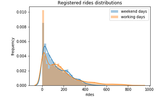
Figure 1.15: The distribution of registered rides: working days versus the weekend
- Perform the same type of hypothesis testing to validate the second assumption from the last section— that is, casual users perform more rides during the weekend. In this case, the null hypothesis is that the average number of rides during working days is the same as the average number of rides during the weekend, both performed only by casual customers. The alternative hypothesis will then result in a statistically significant difference in the average number of rides between the two groups:
# select casual rides for the weekend and working days
weekend_data = preprocessed_data.casual[weekend_mask]
workingdays_data = preprocessed_data.casual[workingdays_mask]
# perform ttest
test_res = ttest_ind(weekend_data, workingdays_data)
print(f"Statistic value: {test_res[0]:.03f}, \
p-value: {test_res[1]:.03f}")
# plot distributions of casual rides for working vs weekend days
sns.distplot(weekend_data, label='weekend days')
sns.distplot(workingdays_data, label='working days')
plt.legend()
plt.xlabel('rides')
plt.ylabel('frequency')
plt.title("Casual rides distributions")
plt.savefig('figs/exercise_1_04_b.png', format='png')
The output should be as follows:
Statistic value: 41.077, p-value: 0.000
The p-value returned from the previous code snippet is 0, which is strong evidence against the null hypothesis. Hence, we can conclude that casual customers also behave differently over the weekend (in this case, they tend to use the bike sharing service more) as seen in the following figure:
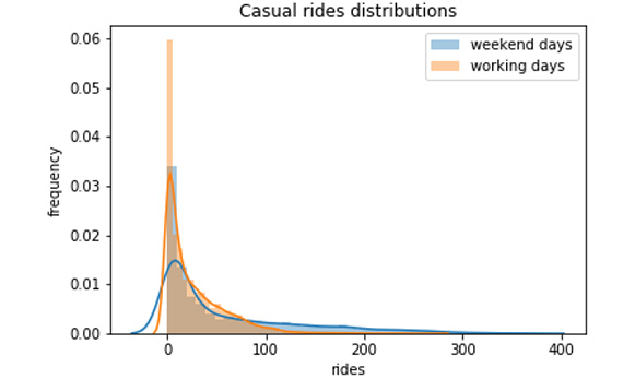
Figure 1.16: Distribution of casual rides: working days versus the weekend
Note
To access the source code for this specific section, please refer to https://packt.live/3fxe7rY.
You can also run this example online at https://packt.live/2C9V0pf. You must execute the entire Notebook in order to get the desired result.
In conclusion, we can say that there is a statistically significant difference between the number of rides on working days and weekend days for both casual and registered customers.