Reader small image

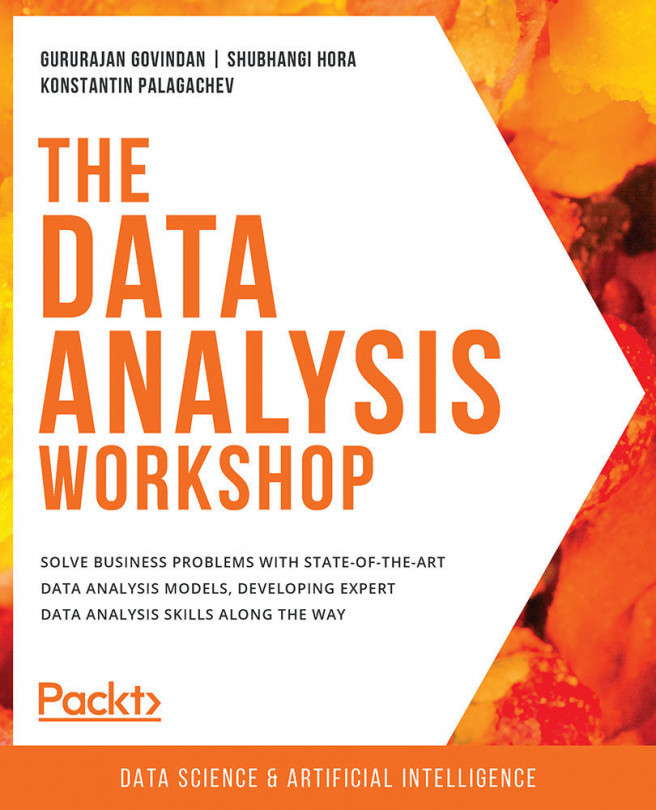
You're reading from  The Data Analysis Workshop

Product typeBook
Published inJul 2020
Reading LevelIntermediate
PublisherPackt
ISBN-139781839211386
Edition1st Edition
Languages
Tools
Concepts
Right arrow
Authors (3):
Gururajan Govindan
Gururajan Govindan
author image
Gururajan Govindan

Gururajan Govindan is a data scientist, intrapreneur, and trainer with more than seven years of experience working across domains such as finance and insurance. He is also an author of The Data Analysis Workshop, a book focusing on data analytics. He is well known for his expertise in data-driven decision-making and machine learning with Python.
Read more about Gururajan Govindan

Shubhangi Hora
Shubhangi Hora
author image
Shubhangi Hora

Shubhangi Hora is a data scientist, Python developer, and published writer. With a background in computer science and psychology, she is particularly passionate about healthcare-related AI, including mental health. Shubhangi is also a trained musician.
Read more about Shubhangi Hora

Konstantin Palagachev
author image
Konstantin Palagachev

Konstantin Palagachev holds a Ph.D. in applied mathematics and optimization, with an interest in operations research and data analysis. He is recognized for his passion for delivering data-driven solutions and expertise in the area of urban mobility, autonomous driving, insurance, and finance. He is also a devoted coach and mentor, dedicated to sharing his knowledge and passion for data science.
Read more about Konstantin Palagachev

View More author details
Right arrow

1. Bike Sharing Analysis

Activity 1.01: Investigating the Impact of Weather Conditions on Rides

  1. Import the required libraries and the initial hour data:
    # import libraries
    import pandas as pd
    import matplotlib.pyplot as plt
    import seaborn as sns
    from scipy.stats import pearsonr
    %matplotlib inline
    # load hourly data
    data = pd.read_csv('https://raw.githubusercontent.com/'\
                       'PacktWorkshops/'\
                       'The-Data-Analysis-Workshop/master/'\
                       'Chapter01/data/hour.csv')
  2. Create a new column in which weathersit is mapped to the four categorical values specified in Exercise 1.01, Preprocessing Temporal and Weather Features...

2. Absenteeism at Work

Activity 2.01: Analyzing the Service Time and Son Columns

  1. First, let's import the data and the necessary libraries:
    # perform statistical test for avg duration difference
    import pandas as pd
    import seaborn as sns
    import matplotlib.pyplot as plt
    %matplotlib inline
    # import data from the github page of the book
    data = pd.read_csv('https://raw.githubusercontent.com/'\
                       'PacktWorkshops/'\
                       'The-Data-Analysis-Workshop/master/'\
                       'Chapter02/data/Absenteeism_at_work.csv', \
                      &...

3. Analyzing Bank Marketing Campaign Data

Activity 3.01: Creating a Leaner Logistic Regression Model

  1. Start by importing the necessary Python packages:
    # import necessary libraries
    import pandas as pd
    import numpy as np
    import statsmodels.api as sm
  2. Load the data from GitHub:
    # pull data from github
    bank_data = pd.read_csv("https://raw.githubusercontent.com/"\
                            "PacktWorkshops/"\
                            "The-Data-Analysis-Workshop/master/"\
                            "Chapter03/data/bank-additional/"\
              ...

4. Tackling Company Bankruptcy

Activity 4.01: Feature Selection with Lasso

  1. Import Lasso from the sklearn.linear_model package:
    from sklearn.linear_model import Lasso
    from sklearn.feature_selection import SelectFromModel
  2. Fit the independent and dependent variables with lasso regularization for the mean_imputed_df4 DataFrame:
    features_names=X6.columns.tolist()
    lasso = Lasso(alpha=0.01 ,positive=True)
    lasso.fit(X6,y6)
  3. Print the coefficients of lasso regularization:
    coef_list=sorted(zip(map(lambda x: round(x,4), \
                             lasso.coef_.reshape(-1)),\
                             features_names), reverse=True)
    coef_list [0:5]

    The output will be as follows:

    [(0.0009, 'X21'), (0.0002, 'X2'), (0.0001, ...

5. Analyzing the Online Shopper's Purchasing Intention

Activity 5.01: Performing K-means Clustering for Administrative Duration versus Bounce Rate and Administrative Duration versus Exit Rate

  1. Select the Administrative Duration and Bounce Rate columns. Assign the column to a variable called x:
    x = df.iloc[:, [1, 6]].values
    x.shape
  2. Initialize the k-means algorithm:
    wcss = []
    for i in range(1, 11):
        km = KMeans(n_clusters = i, init = 'k-means++', \
                    max_iter = 300, n_init = 10, random_state = 0, \
                    algorithm = 'elkan', tol = 0.001)
  3. For the different values of K, compute the Kmeans inertia and store it in a variable called wcss:
        km.fit(x)
        labels = km.labels_
        wcss.append...

6. Analysis of Credit Card Defaulters

Activity 6.01: Evaluating the Correlation between Columns Using a Heatmap

  1. Plot the heatmap for all the columns in the DataFrame (other than the ID column) by using sns.heatmap and keep the figure size as 30,10 for better visibility:
    sns.set(rc={'figure.figsize':(30,10)})
    sns.set_context("talk", font_scale=0.7)
  2. Use Spearman as the method parameter to compute Spearman's rank correlation coefficient:
    sns.heatmap(df.iloc[:,1:].corr(method='spearman'), \
                cmap='rainbow_r', annot=True)

    The output of the heatmap is as follows:

    Figure 6.28: Heatmap for Spearman's rank correlation

  3. In order to get the exact correlation coefficients of each column with the DEFAULT column, apply the .corr() function on each column with respect to the DEFAULT column:
    df.drop("DEFAULT", axis=1)\
    .apply(lambda x: x.corr(df.DEFAULT...

7. Analyzing the Heart Disease Dataset

Activity 7.01: Checking for Outliers

  1. Plot a box plot using sns.boxplot for the st_depr column:
    sd = sns.boxplot(df['st_depr'])
    plt.show()

    The output will be as follows:

    Figure 7.22: Box plot for st_depr

    Figure 7.22: Box plot for st_depr

  2. Plot a box plot using sns.boxplot for the colored_vessels column:
    cv = sns.boxplot(df['colored_vessels'])
    plt.show()

    The output will be as follows:

    Figure 7.23: Boxplot for colored_vessels

    Figure 7.23: Boxplot for colored_vessels

  3. Plot a box plot using sns.boxplot for the thalassemia column:
    t = sns.boxplot(df['thalassemia'])
    plt.show()

    The output will be as follows:

    Figure 7.24: Boxplot for thalassemia

Figure 7.24: Boxplot for thalassemia

Note

To access the source code for this specific section, please refer to https://packt.live/2N4I0DF.

You can also run this example online at https://packt.live/2BiGv2c. You must execute the entire Notebook in order to get the desired result.

Activity 7.02: Plotting Distributions and Relationships between Columns with Respect to the...
8. Analyzing Online Retail II Dataset

Activity 8.01: Performing Data Analysis on the Online Retail II Dataset

  1. Import the required packages:
    import pandas as pd
    import numpy as np
    import seaborn as sns
    import matplotlib.pyplot as plt

    In a Jupyter notebook, install plotly using the following command:

    !pip install plotly

    Import plotly.express from the installed package:

    import plotly.express as px
  2. Store each of the CSV files in two different DataFrames:
    r09 = pd.read_csv('https://raw.githubusercontent.com/'\
                      'PacktWorkshops/'\
                      'The-Data-Analysis-Workshop/master/'\
                      'Chapter08/Datasets/online_retail_II.csv')
    r09.head()

    The output...

9. Analysis of the Energy Consumed by Appliances

Activity 9.01: Analyzing the Appliances Energy Consumption

  1. Using seaborn, plot a boxplot for the a_energy column:
    app_box = sns.boxplot(new_data.a_energy)

    The output will be as follows:

    Figure 9.28: Box plot of a_energy

    Figure 9.28: Box plot of a_energy

  2. Use .sum() to determine the total number of instances wherein the value of the energy consumed by appliances is above 200 Wh:
    out = (new_data['a_energy'] > 200).sum()
    out

    The output will be as follows:

    1916
  3. Calculate the percentage of the number of instances wherein the value of the energy consumed by appliances is above 200 Wh:
    (out/19735) * 100

    The output will be as follows:

    9.708639473017481
  4. Use .sum() to check the total number of instances wherein the value of the energy consumed by appliances is above 950 Wh:
    out_e = (new_data['a_energy'] > 950).sum()
    out_e

    The output will be as follows:

    2
  5. Calculate the percentage of the number of instances wherein the value of the energy consumed...

10. Analyzing Air Quality

Activity 10.01: Checking for Outliers

  1. Plot a boxplot for the PM25 feature using seaborn:
    pm_25 = sns.boxplot(air['PM25'])

    The output will be as follows:

    Figure 10.50: Boxplot for PM25

    Figure 10.50: Boxplot for PM25

  2. Check how many instances contain values of PM25 higher than 250:
    (air['PM25'] >= 250).sum()

    The output will be as follows:

    18668
  3. Store all the instances from Step 2 in a DataFrame called pm25 and print the first five rows:
    pm25 = air.loc[air['PM25'] >= 250]
    pm25.head()

    The output will be as follows:

    Figure 10.51: First five rows of pm25

    Figure 10.51: First five rows of pm25

  4. Print the station names of the instances in PM25 to ensure all the instances are not just from one station, but from multiple stations. This reduces the chances of them being incorrectly stored values:
    pm25.station.unique()

    The output will be as follows:

    array(['Aotizhongxin', 'Changping', 'Dingling', 'Dongsi', 
           &apos...
lock icon
The rest of the chapter is locked
You have been reading a chapter from
The Data Analysis Workshop
Published in: Jul 2020Publisher: PacktISBN-13: 9781839211386
Register for a free Packt account to unlock a world of extra content!
A free Packt account unlocks extra newsletters, articles, discounted offers, and much more. Start advancing your knowledge today.
undefined
Unlock this book and the full library FREE for 7 days
Get unlimited access to 7000+ expert-authored eBooks and videos courses covering every tech area you can think of
Renews at $15.99/month. Cancel anytime

Authors (3)

author image
Gururajan Govindan

Gururajan Govindan is a data scientist, intrapreneur, and trainer with more than seven years of experience working across domains such as finance and insurance. He is also an author of The Data Analysis Workshop, a book focusing on data analytics. He is well known for his expertise in data-driven decision-making and machine learning with Python.
Read more about Gururajan Govindan

author image
Shubhangi Hora

Shubhangi Hora is a data scientist, Python developer, and published writer. With a background in computer science and psychology, she is particularly passionate about healthcare-related AI, including mental health. Shubhangi is also a trained musician.
Read more about Shubhangi Hora

author image
Konstantin Palagachev

Konstantin Palagachev holds a Ph.D. in applied mathematics and optimization, with an interest in operations research and data analysis. He is recognized for his passion for delivering data-driven solutions and expertise in the area of urban mobility, autonomous driving, insurance, and finance. He is also a devoted coach and mentor, dedicated to sharing his knowledge and passion for data science.
Read more about Konstantin Palagachev