Power BI Desktop contains a rich set of connectors and transformation capabilities that support the integration and enhancement of data from many different sources. These features are all driven by a powerful functional language and query engine, M, which leverages source system resources when possible and can greatly extend the scope and robustness of the data retrieval process beyond what's possible via the standard query editor interface alone. As with almost all BI projects, the design and development of the data access and retrieval process has significant implications for the analytical value, scalability, and sustainability of the overall Power BI solution.

In this chapter, we dive into Power BI Desktop's Get Data experience and walk through the process of establishing and managing data source connections and queries. Examples are provided of using the Power Query Editor interface and the M language directly, to construct and refine queries to meet common data transformation and cleansing needs. In practice and as per the examples, a combination of both tools is recommended to aid the query development process.

A full explanation of the M language and its implementation in Power BI is outside the scope of this book, but additional resources and documentation are included in the sections titled There's more... and See also.

The recipes included in this chapter are as follows:

• Viewing and Analyzing M Functions
• Managing Queries and Data Sources
• Using DirectQuery
• Importing Data
• Applying Multiple Filters
• Selecting and Renaming Columns
• Transforming and Cleansing Source Data
• Creating Custom Columns
• Combining and Merging Queries
• Selecting Column Data Types
• Visualizing the M Library
• Profile Source Data
• Diagnosing Queries

The following are required to complete the recipes in this chapter:

• Power BI Desktop
• SQL Server 2019 or newer with the AdventureWorksDW2019 database installed. This database and instructions for installing it are available here: http://bit.ly/2OVQfG7

Every time you click on a button to connect to any of Power BI Desktop's supported data sources or apply any transformation to a data source object, such as changing a column's data type, one or multiple M expressions are created reflecting your choices. These M expressions are automatically written to dedicated M documents and, if saved, are stored within the Power BI Desktop file as Queries. M is a functional programming language like F#, and it is important that Power BI developers become familiar with analyzing, understanding, and later, writing and enhancing the M code that supports their queries.

Getting ready

To prepare for this recipe, we will first build a query through the user interface that connects to the AdventureWorksDW2019 SQL Server database, retrieves the DimGeography table, and then filters this table to a single country, such as the United States:

1. Open Power BI Desktop and click on Get Data from the Home tab of the ribbon. Select SQL Server from the list of database sources. For future reference, if the data source is not listed in Common data sources, more data sources are available by clicking More… at the bottom of the list.
2. A dialog window is displayed asking for connectivity information. Ensure that Data Connectivity mode is set to Import. Enter the name of your SQL server as well as the AdventureWorksDW2019 database. In Figure 2.1, my SQL server is installed locally and running under the instance MSSQLSERVERDEV. Thus, I set the server to be localhost\MSSQLSERVERDEV to specify both the server (localhost) and the instance. If you leave the Database field blank, this will simply result in an extra navigation step to select the desired database.

   

   Figure 2.1: SQL Server Get Data dialog

3. If this is the first time connecting to this database from Power BI, you may be prompted for some credentials. In addition, you may also be warned that an encrypted connection cannot be made to the server. Simply enter the correct credentials for connecting and click the Connect button. For the encryption warning, simply click the OK button to continue.
4. A navigation window will appear, with the different objects and schemas of the database. Select the DimGeography table from the Navigator window and click the Transform Data button.
5. The Power Query Editor launches in a new window with a query called DimGeography; preview data from that table is displayed in the center of the window. In the Power Query Editor window, use the scroll bar at the bottom of the central display area to find the column called EnglishCountryRegionName. You can also select a column and then click Go to Column in the ribbon of the View menu to search for and navigate to a column quickly. Click the small button in the column header next to this column to display a sorting and filtering drop-down menu.

   Uncheck the (Select All) option to deselect all values and then check the box next to a country, such as the United States, before clicking the OK button.

   

Figure 2.2: Filtering for United States only in the Query Editor

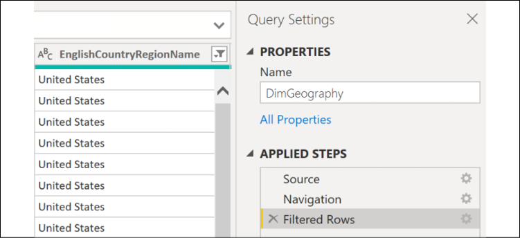
Note that the button for the EnglishCountryRegionName column changes to display a funnel icon. Also notice that, in the Query Settings pane on the right side of the window, a new option under APPLIED STEPS has appeared called Filtered Rows.

Figure 2.3: The Query Settings pane in the Query Editor

How to View and Analyze M Functions

There are two methods for viewing and analyzing the M functions comprising a query; they are as follows:

• Formula bar
• Advanced Editor

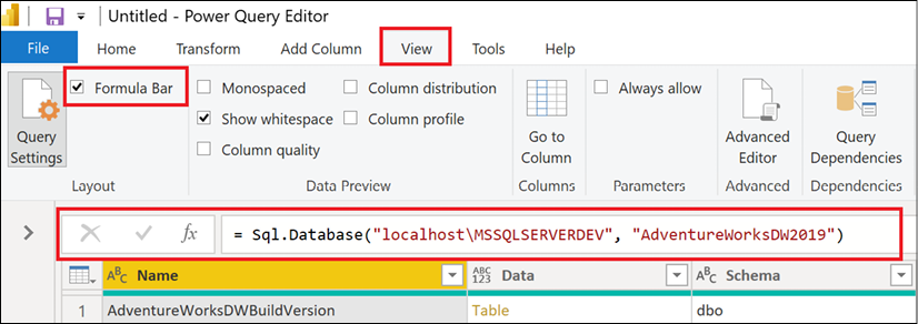
The formula bar exposes the M function for the current step only. This formula bar appears just above the column headers for the preview data in the central part of the window. If you do not see this formula bar, click the View tab and check the box next to Formula Bar in the Layout section of the ribbon. All such areas of interest are boxed in red in Figure 2.4.

Figure 2.4: The Power Query Editor formula bar

When the Source step is selected under APPLIED STEPS in the Query Settings pane, as seen in Figure 2.3, we see the connection information specified on the initial dialog after selecting Get Data and then SQL Server. The M function being used is Sql.Database. This function is accepting two parameters: the server name, localhost\MSSQLSERVERDEV, and the database name, AdventureWorksDW2019. Clicking on other steps under APPLIED STEPS exposes the formulas for those steps, which are technically individual M expressions.

The formula bar is useful to quickly understand the M code behind a particular query step. However, it is more convenient and often essential to view and edit all the expressions in a centralized window. This is the purpose of the Advanced Editor. To launch the Advanced Editor, follow these steps:

1. Click on the Home tab and then select Advanced Editor from the Query section of the ribbon, as shown in Figure 2.5. Alternatively, the Advanced Editor can also be accessed from the View tab, shown in Figure 2.4.

   

   Figure 2.5: Advanced Editor on the Home tab of the Query Editor

2. The Advanced Editor dialog is displayed, exposing all M functions and comments that comprise the query. The M code can be directly edited from within this dialog.

   

Figure 2.6: The Advanced Editor view of the DimGeography query

As shown in Figure 2.6, using the Advanced Editor will mean that all of the Power Query code that comprises the query can be viewed in one place.

How it works

The majority of queries created for Power BI follow the let...in structure, as per this recipe. Within the let block, there are multiple steps with dependencies among those steps. For example, the second step, dbo_DimGeography, references the previous step, Source. Individual expressions are separated by commas, and the expression referred to following the in keyword is the expression returned by the query. The individual step expressions are technically known as "variables".

Variable names in M expressions cannot have spaces without being preceded by a hash sign and enclosed in double quotes. When the Query Editor graphical interface is used to create M queries, this syntax is applied automatically, along with a name describing the M transformation applied. This behavior can be seen in the Filtered Rows step in Figure 2.6. Applying short, descriptive variable names (with no spaces) improves the readability of M queries.

Note the three lines below the let statement. These three lines correspond to the three APPLIED STEPS in our query: Source, Navigation, and Filtered Rows. The query returns the information from the last step of the query, Filtered Rows. As more steps are applied, these steps will be inserted above the in statement and the line below this will change to reference the final step in the query.

M is a case-sensitive language. This includes referencing variables in M expressions (RenameColumns versus Renamecolumns) as well as the values in M queries. For example, the values "Apple" and "apple" are considered unique values in an M query.

It is recommended to use the Power Query Editor user interface when getting started with a new query and when learning the M language. After several steps have been applied, use Advanced Editor to review and optionally enhance or customize the M query. As a rich, functional programming language, there are many M functions and optional parameters not exposed via the Power Query Editor's graphical user interface. Going beyond the limits of the Power Query Editor enables more robust data retrieval, integration, and data mashup processes.

The M engine also has powerful "lazy evaluation" logic for ignoring any redundant or unnecessary variables, as well as short-circuiting evaluation (computation) once a result is determinate, such as when one side (operand) of an OR logical operator is computed as True. Lazy evaluation allows the M query engine to reduce the required resources for a given query by ignoring any unnecessary or redundant steps (variables). The order of evaluation of the expressions is determined at runtime—it doesn't have to be sequential from top to bottom.

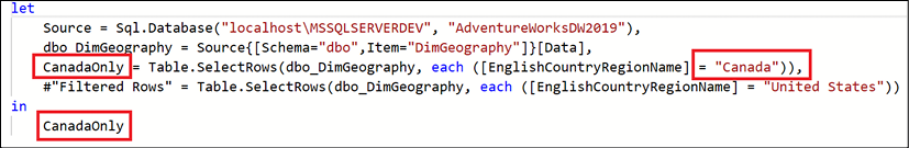
In the following example, presented in Figure 2.7, a step for retrieving Canada was added and the "Filtered Rows" step for filtering the results for the United States was ignored. Since the CanadaOnly variable satisfies the overall let expression of the query, only the Canada query is issued to the server as if the "Filtered Rows" step were commented out or omitted.

Figure 2.7: Revised query that ignores the "Filtered Rows" step to evaluate Canada only

As a review of the concepts covered thus far and for future reference, Table 2.1 presents a glossary of the main concepts of the M language utilized in this book.

Table 2.1: M Language elements

There's more...

M queries are not intended as a substitute for the data loading and transformation workloads typically handled by enterprise data integration and orchestration tools such as Azure Data Factory (ADF), Azure Databricks, or SQL Server Integration Services (SSIS). However, just as BI professionals carefully review the logic and test the performance of SQL stored procedures and ETL packages supporting their various cubes and reporting environments, they should also review the M queries created to support Power BI models and reports. When developing retrieval processes for Power BI models, consider these common ETL questions:

• How are queries impacting the source systems?
• Can we make our queries more resilient to changes in source data so that they avoid failure?
• Are our queries efficient and simple to follow and support, or are there unnecessary steps and queries?
• Are our queries delivering sufficient performance to the BI application?
• Is our process flexible, such that we can quickly apply changes to data sources and logic?
• Can some or all of the required transformation logic be implemented in a source system such as the loading process for a data warehouse table or a SQL view?

One of the top performance and scalability features of M's query engine is called Query Folding. If possible, the M queries developed in Power BI Desktop are converted ("folded") into SQL statements and passed to source systems for processing.

If we use the original version of the query from this recipe, as shown in Figure 2.6, we can see Query Folding in action. The query from this recipe was folded into the following SQL statement and sent to the server for processing, as opposed to the M query engine performing the processing locally. To see how this works, perform the following:

1. Right-click on the Filtered Rows step in the APPLIED STEPS section of the Query Settings pane, and select View Native Query.

   

   Figure 2.8: View Native Query in Query Settings

2. The Native Query dialog is then displayed, as shown in Figure 2.9.

   

Figure 2.9: The SQL statement generated from the DimGeography M query

Finding and revising queries that are not being folded to source systems is a top technique for enhancing large Power BI datasets. See the Pushing Query Processing Back to Source Systems recipe of Chapter 11, Enhancing and Optimizing Existing Power BI Solutions, for an example of this process.

The M query engine also supports partial query folding. A query can be "partially folded", in which a SQL statement is created resolving only part of an overall query. The results of this SQL statement would be returned to Power BI Desktop (or the on-premises data gateway) and the remaining logic would be computed using M's in-memory engine with local resources. M queries can be designed to maximize the use of the source system resources, by using standard expressions supported by query folding early in the query process. Minimizing the use of local or on-premises data gateway resources is a top consideration for improving query performance.

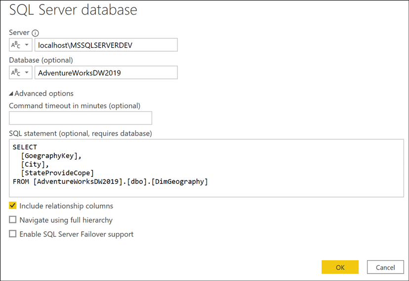
There are limits, however, to query folding. For example, no folding takes place once a native SQL query has been passed to the source system, such as when passing a SQL query directly through the Get Data dialog using the Advanced options. Figure 2.10 displays a query specified in the Get Data dialog, which is included in the Source step.

Figure 2.10: Providing a user-defined native SQL query

Any transformations applied after this native query will use local system resources. Therefore, the general implication for query development with native or user-defined SQL queries is that if they are used, try to include all required transformations (that is, joins and derived columns), or use them to utilize an important feature of the source database that is not being utilized by the folded query, such as an index.

Some other things to keep in mind regarding Query Folding are the following:

• Not all data sources support Query Folding, such as text and Excel files.
• Not all transformations available in the Query Editor or via M functions are directly supported by some data sources.
• The privacy levels defined for the data sources will also impact whether folding is used or not.
• SQL statements are not parsed before they are sent to the source system.
• The Table.Buffer function can be used to avoid query folding. The table output of this function is loaded into local memory, and transformations against it will remain local.

See also

• Power Query M language specification: http://bit.ly/2oaJWwv
• Power Query M Function reference: http://bit.ly/3bLKJ1M

There are two primary components of queries in Power BI: the data source and the query logic executed against this source. The data source includes the connection method (DirectQuery or Import), a privacy setting, and the authentication credentials. The query logic consists of the M expressions represented as queries in the Query Editor and stored internally as M documents.

In a typical corporate BI tool, such as SQL Server Reporting Services (SSRS), the properties of a data source such as the server and database name are defined separately from the queries that reference them. In Power BI Desktop, however, by default, each individual query created explicitly references a given data source (for example, server A and database B). This creates an onerous, manual process of revising each query if it becomes necessary to change the source environment or database.

This issue is addressed in the following steps by using dedicated M queries to centralize and isolate the data source information from the individual queries. Additionally, detail and reference information is provided on managing source credentials and data source privacy levels.

Getting ready

To prepare for this recipe, we will create a query from a database, which will serve as the source for other queries via the standard Get Data and Power Query Editor experience described in the previous recipe. To create this query, perform the following steps:

1. Open Power BI Desktop.
2. If you have already connected to your SQL Server, you can find the connection under Recent sources on the Home tab. Otherwise, on the Home tab, select Get Data from the ribbon, and choose SQL Server.
3. Select a table or view, and click on Transform Data to import the data.
4. The Power Query Editor window will launch and a preview of the data will appear. In this example, we have chosen the DimEmployee table from the AdventureWorksDW2019 database on our local SQL Server instance MSSQLSERVERDEV. The full code of the query can be viewed in the Advanced Editor window but is also shown below.

   let
       Source = Sql.Database("localhost\MSSQLSERVERDEV", "AdventureWorksDW2019"),
       dbo_DimEmployee = Source{[Schema="dbo",Item="DimEmployee"]}[Data]
   in
       dbo_DimEmployee
   

5. Copy just the Source line (in bold in the previous step).
6. Close the Advanced Editor window by clicking the Cancel button.
7. Remain in the Power Query Editor window.

How to Manage Queries and Data Sources

In this example, a separate data source connection query is created and utilized by individual queries. By associating many individual queries with a single (or a few) data source queries, it is easy to change the source system or environment, such as when switching from a Development environment to a User Acceptance Testing (UAT) environment. We will then further separate out our data source queries and our data load queries using query groups. To start isolating our data source queries from our data load queries, follow these steps:

1. Create a new, blank query by selecting New Source from the ribbon of the Home tab and then select Blank Query.
2. Open the Advanced Editor and replace the Source line with the line copied from the query created in Getting ready. Be certain to remove the comma (,) at the end of the line. The line prior to the in keyword should never have a comma at the end of it. Your query should look like the following:

   let
       Source = Sql.Database("localhost\MSSQLSERVERDEV", "AdventureWorksDW2019")
   in
       Source
   

3. Click the Done button to close the Advanced Editor window.
4. Rename the query by clicking on the query and editing the Name in the Query Settings pane. Alternatively, in the Queries pane, right-click the query and choose Rename. Give the source query an intuitive name, such as AdWorksDW.
5. Now click on the original query created in the Getting ready section above. Open the Advanced Editor. Replace the Source step expression of the query with the name of the new query. As you type the name of the query, AdWorksDW, you will notice that IntelliSense will suggest possible values. The query should now look like the following:

   let
       Source = AdWorksDW,
       dbo_DimEmployee = Source{[Schema="dbo",Item="DimEmployee"]}[Data]
   in
       dbo_DimEmployee
   

6. Click the Done button to come out of Advanced Editor. The preview data refreshes but continues to display the same data as before.

We can take this concept of isolating our data source queries from data loading queries further by organizing our queries into query groups. You should also use query groups to help isolate data source and staging queries from queries loaded to the dataset. To see how query groups work, follow these steps:

1. Duplicate the revised data loading query that loads the DimEmployee table, created in Getting ready. Simply right-click the query in the Queries pane and choose Duplicate.
2. With the new query selected in the Queries pane, click the gear icon next to the Navigation step in the APPLIED STEPS area of the Query Settings pane.
3. Choose a different dimension table or view, such as DimAccount, and then click the OK button. Dimension tables and views start with "Dim".
4. Rename this new query to reflect the new table or view being loaded.
5. Create a new group by right-clicking in a blank area in the Queries window and then selecting New Group…
6. In the New Group dialog, name the group Data Sources and click the OK button.
7. Create another new group and name this group Dimensions.
8. Move the AdWorksDW query to the Data Sources group by either dragging and dropping in the Queries pane or right-clicking the query and choosing Move To Group…, and then select the group.
9. Move the other queries to the Dimensions group.
10. Finally, ensure that the query in the Data Source group is not actually loaded as a separate table in the data model. Right-click on the query and uncheck the Enable Load option. This makes the query available to support data retrieval queries but makes the query invisible to the model and report layers. The query name will now be italicized in the Queries pane.

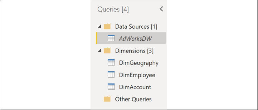
Your Queries pane should now look similar to that in Figure 2.11:

Figure 2.11: Queries organized into query groups

How it works

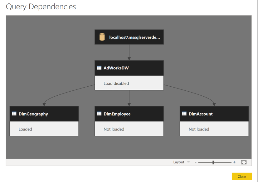
The Query Dependencies view in Power Query provides a visual representation of the relationships between the various queries. You can access this dialog by using the View tab and then selecting Query Dependencies in the ribbon.

Figure 2.12: The Query Dependencies View in Query Editor

In this example, a single query with only one expression is used by multiple queries, but more complex interdependencies can be designed to manage the behavior and functionality of the retrieval and analytical queries. This recipe illustrates the broader concept used in later recipes called "composability", where functions call other functions; this is one of the primary strengths of functional programming languages such as M, DAX, R, and F#.

There's more...

Power BI Desktop saves data source credentials for each data source defined, as well as a privacy level for that source. It is often necessary to modify these credentials as passwords change. In addition, setting privacy levels on data sources helps prevent confidential information from being exposed to external sources during the Query Folding process. Data source credentials and settings are not stored in the PBIX file, but rather on the computer of the installed application.

To manage data source credentials and privacy levels, perform the following steps:

1. From Power BI Desktop (not the Power Query Editor), click on File in the menu, then click Options and settings, and finally click Data source settings.
2. Click on the Global Permissions radio button such that your settings are persisted into other Power BI Desktop reports.
3. Select a data source.
4. Click the Edit Permissions button.
5. From the Edit Permissions dialog, you can click the Edit button under the Credentials heading to set the authentication credentials for the data source. In addition, you can set the privacy level for the data source using the drop-down under the Privacy Level heading. Click OK to save your settings.

   

Figure 2.13: Edit credentials and privacy level for a data source

Definitions of the available Privacy Level settings are provided in Table 2.2.

Table 2.2: Privacy Level Settings

Just as relational databases such as SQL Server consider many potential query plans, the M engine also searches for the most efficient methods of executing queries, given that the data sources and query logic are defined. In the absence of data source privacy settings, the M engine is allowed to consider plans that merge disparate data sources. For example, a local text file of customer names can be merged with an external or third-party server, given the better performance of the server. Defining privacy settings isolates data sources from these operations thus increasing the likelihood of local resource usage, and hence query performance may be reduced.

See also

• Authentication with a data source: http://bit.ly/30It2tV
• Power BI Desktop privacy levels: http://bit.ly/29blFBR

One of the most valuable features of Power BI is its deep support for real-time and streaming datasets, with the ability to provide immediate visibility to business processes and events as this data is created or updated. As Power BI Desktop's data modeling engine reflects the latest Analysis Services features, it becomes feasible to design DirectQuery models or composite models (DirectQuery and import) in Power BI Desktop, and thus avoid the scalability limitations and scheduled refresh requirements of models based on importing data.

The three most common candidates for DirectQuery or composite model projects are as follows:

• The data model would consume an exorbitant amount of memory if all tables were fully loaded into memory. Even if the memory size is technically supported by large Power BI Premium capacity nodes, this would be a very inefficient and expensive use of company resources as most BI queries only access aggregated data representing a fraction of the size. Composite models which mix DirectQuery and Dual storage mode tables with in-memory aggregation tables is the recommended architecture for large models going forward.
• Access to near-real-time data is of actionable or required value to users or other applications, such as is the case with notifications. For example, an updateable Nonclustered Columnstore index could be created on OLTP disk-based tables or memory-optimized tables in SQL Server to provide near-real-time access to database transactions.
• A high-performance and/or read-optimized system is available to service report queries, such as a SQL Server or Azure SQL Database, with the Clustered Columnstore index applied to fact tables.

This recipe walks through the primary steps in designing the data access layer that supports a DirectQuery model in Power BI Desktop. As these models are not cached into memory and dynamically convert the DAX queries from report visualizations to SQL statements, guidance is provided to maintain performance. Additional details, resources, and documentation on DirectQuery's current limitations and comparisons with the default import mode are also included to aid your design decision.

Getting ready

1. Choose a database to serve as the source for the DirectQuery data model.
2. Create a logical and physical design of the fact and dimension tables of the model including the relationship keys and granularity of the facts. The AdventureWorksDW database is a good example of data designed in this manner.
3. Determine or confirm that each fact-to-dimension relationship has referential integrity. Providing this information to the DirectQuery model allows for more performant inner join queries.
4. Create view objects in the source database to provide efficient access to the dimensions and facts defined in the physical design.

Be aware that DirectQuery models are limited to a single source database and not all databases are supported for DirectQuery. If multiple data sources are needed, such as SQL Server and Oracle, or Teradata and Excel, then the default Import mode model, with a scheduled refresh to the Power BI Service, will be the only option.

How to use DirectQuery

For this recipe, we will use the AdventureWorksDW2019 database that has been used thus far in this chapter. To implement this recipe, follow these steps:

1. Create a new Power BI Desktop file.
2. From the Home tab, click on Get Data in the ribbon and then SQL Server.
3. In the Data Connectivity mode section, choose the DirectQuery radio option.

   

   Figure 2.14: Creating a DirectQuery data source

4. Select a table or view to be used by the model via the Navigator dialog, such as the FactResellerSales table, and then click the Transform Data button.
5. Duplicate the initial query and revise the Navigation step to reference an additional view supporting the model, such as the DimReseller. This can be done by editing the Item in the formula bar or by clicking on the gear icon next to the Navigation step under APPLIED STEPS in the Query Settings pane. Also, rename this query to reflect the data being referenced.

   

   Figure 2.15: Editing the Navigation step in the formula bar

6. Repeat step 5 for all required facts and dimensions. For example:
   • DimEmployee
   • DimPromotion
   • DimCurrency
   • DimSalesTerritory
7. Click the Close and Apply button.

The Report Canvas view will confirm that the model is in DirectQuery mode via the status bar at the bottom right (see Figure 2.16). In addition, the Data view in the left-hand pane, which is visible for import models, will not be visible.

Figure 2.16: DirectQuery Status in Power BI Desktop

How it works

The M transformation functions supported in DirectQuery are limited by compatibility with the source system. The Power Query Editor will advise when a transformation is not supported in DirectQuery mode, per Figure 2.17.

Figure 2.17: A warning in Query Editor that the IsEven function is not supported in DirectQuery mode

Given this limitation and the additional complexity the M-based transforms would add to the solution, it is recommended that you embed all the necessary logic and transforms in the source relational layer. Ideally, the base tables in the source database themselves would reflect these needs. As a secondary option, a layer of views can be created to support the DirectQuery model.

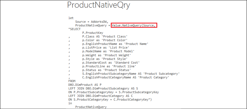
If the database objects themselves cannot be revised, the Value.Native M function can be used to directly pass the SQL statement from Power BI Desktop to the source database, as per Figure 2.18.

Figure 2.18: The Value.Native function used to pass a SQL statement to a source system

As report visualizations are refreshed or interacted with in Power BI, the DAX queries from each visualization are translated into SQL statements, utilizing the source SQL statements to return the results. Be aware that Power BI does cache query results with DirectQuery models. Therefore, when accessing a recently utilized visual, a local cache may be used rather than a new query sent to the source.

The SQL statements passed from Power BI to the DirectQuery data source include all columns from the tables referenced by the visual.

For example, a Power BI visual with SalesAmount from the FactResellerSales table grouped by ResellerName from DimReseller would result in a SQL statement that selects the columns from both tables and implements the join defined in the model. However, as the SQL statement passed embeds these source views as derived tables, the relational engine is able to generate a query plan that only scans the required columns to support the join and aggregation.

There's more...

The performance and scalability of DirectQuery models are primarily driven by the relational data source. A denormalized star schema with referential integrity and a system that is isolated from OLTP workloads is recommended if near real-time visibility is not required. Additionally, in-memory and columnar features available to supported DirectQuery sources are recommended for reporting and analytical queries.

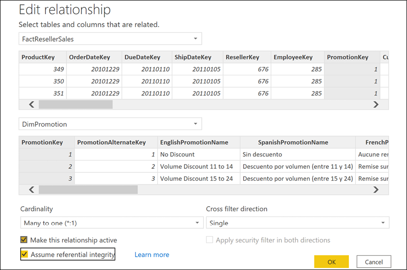
By default, DirectQuery models generate outer join SQL queries to ensure that measures return the correct value even if there's not a related dimension. However, you can configure DirectQuery models to send inner join queries. This is done by editing the relationship between tables in the modeling view by checking the Assume referential integrity setting (see Figure 2.19). Along with source system resources, this is one of the top factors contributing to the DirectQuery model's performance.

Figure 2.19: Activating referential integrity assumption in relationships

Of course, you should ensure that there is referential integrity in the source before enabling this setting; otherwise, incorrect results could be returned.

The design of the source relational schema and the hardware resources of this system can, of course, greatly impact the performance of DirectQuery models.

A classic star-schema design with denormalized tables is recommended to reduce the required join operations at query time. Optimizing relational fact tables with column store technologies such as the Clustered Columnstore Index for SQL Server and table partitions will also significantly benefit DirectQuery models.

See also

• Power BI Desktop DirectQuery documentation: http://bit.ly/2nUoLOG
• The Power BI data sources documentation provides a detailed list of data sources broken down by the connectivity options supported: http://bit.ly/30N5ofG

Import is the default data connectivity mode for Power BI Desktop. Import models created in Power BI Desktop use the same in-memory, columnar compressed storage engine (VertiPaq) featured in Analysis Services Tabular 2016+ import models. Import mode models support the integration of disparate data sources (for example, SQL Server and DB2) and allow more flexibility in developing metrics and row-level security roles via full support for all DAX functions.

There are some limits for Import mode datasets, however. For example, Power BI Pro license users cannot publish Power BI Desktop files to shared capacity in the Power BI service that are larger than 1GB. Power BI Premium (dedicated, isolated hardware) supports datasets of 10GB in size and larger (with large datasets enabled, dataset size is limited by the Premium capacity size or the maximum size set by the administrator). With such large datasets, it is important to consider employing incremental refresh where only new and changed data is refreshed and imported, instead of the entire dataset being refreshed.

This recipe describes a process of using M and the Query Editor to develop the Import mode queries for a standard star-schema analytical model. A staging query approach is introduced as a means of efficiently enhancing the dimensions of a model. In addition, tips are included for using fewer resources during the refresh and avoiding refresh failures from revised source data. More details of these methods are included in other recipes in this chapter.

Getting ready

In this example, the DimProduct, DimProductSubcategory, and DimProductCategory tables from the AdventureWorksDW2019 database are integrated into a single import query. This query includes all product rows, only the English language columns, and user-friendly names. Many-to-one relationships have been defined in the source database.

To prepare for this recipe, do the following:

1. Open Power BI Desktop.
2. Create an Import mode data source query called AdWorksDW. This query should be similar to the following:

   let
       Source = Sql.Database("localhost\MSSQLSERVERDEV", "AdventureWorksDW2019")
   in
       Source
   

3. Isolate this query in a query group called Data Sources.
4. Disable loading of this query.

For additional details on performing these steps, see the Managing Queries and Data Sources recipe in this chapter.

How to import data

To implement this recipe, perform the following steps:

1. Right-click AdWorksDW and choose Reference. This creates a new query that references the AdWorksDW query as its source.
2. Select this new query and, in the preview data, find the DimProduct table in the Name column. Click on the Table link in the Data column for this row.
3. Rename this query DimProduct.
4. Repeat steps 1 – 3 for the DimProductCategory and DimProductSubcategory tables.
5. Create a new query group called Staging Queries.
6. Move the DimProduct, DimProductCategory, and DimProductSubcategory queries to the Staging Queries group.
7. Disable loading for all queries in the Staging Queries group. Your finished set of queries should look similar to Figure 2.20.

   

   Figure 2.20: Staging Queries

   The italics indicate that the queries will not be loaded into the model.

8. Create a new Blank Query and name this query Products.
9. Open the Advanced Editor for the Products query.
10. In the Products query, use the Table.NestedJoin function to join the DimProduct and DimProductSubcategory queries. This is the same function that is used if you were to select the Merge Queries option in the ribbon of the Home tab. A left outer join is required to preserve all DimProduct rows, since the foreign key column to DimProductCategory allows null values.
11. Add a Table.ExpandColumns expression to retrieve the necessary columns from the DimProductSubcategory table. The Products query should now have the following code:

    let
        ProductSubCatJoin = 
            Table.NestedJoin(
                DimProduct,"ProductSubcategoryKey",
                DimProductSubcategory,"ProductSubcategoryKey",
                "SubCatColumn",JoinKind.LeftOuter
            ),
        ProductSubCatColumns =
            Table.ExpandTableColumn(
                ProductSubCatJoin,"SubCatColumn",
                {"EnglishProductSubcategoryName","ProductCategoryKey"},
                {"Product Subcategory", "ProductCategoryKey"}
            )
    in
        ProductSubCatColumns
    

    The NestedJoin function inserts the results of the join into a column (SubCatColumn) as table values. The second expression converts these table values into the necessary columns from the DimProductSubcategory query and provides the simple Product Subcategory column name, as shown in Figure 2.21.

    

    Figure 2.21: Product Subcategory Columns Added

    The query preview in the Power Query Editor will expose the new columns at the far right of the preview data.

12. Add another expression beneath the ProductSubCatColumns expression with a Table.NestedJoin function that joins the previous expression (the Product to Subcategory join) with the DimProductCategory query.
13. Just like step 8, use a Table.ExpandTableColumn function in a new expression to expose the required Product Category columns.

            ),
        
        ProductCatJoin = 
            Table.NestedJoin(
                ProductSubCatColumns,"ProductCategoryKey",
                DimProductCategory,"ProductCategoryKey",
                "ProdCatColumn",JoinKind.LeftOuter
            ),
        ProductCatColumns = 
            Table.ExpandTableColumn(
                ProductCatJoin,"ProdCatColumn",
                {"EnglishProductCategoryName"}, {"Product Category"}
            )
    in
        ProductCatColumns
    

    Be certain to add a comma after the ProductSubCatColumns expression. In addition, be sure to change the line beneath the in keyword to ProductCatColumns.

    The expression ProductCatJoin adds the results of the join to DimProductCategory (the right table) to the new column (ProdCatColumn). The next expression, ProductCatColumns adds the required Product Category columns and revises the EnglishProductCategoryName column to Product Category. A left outer join was necessary with this join operation as well since the product category foreign key column on DimProductSubcategory allows null values.

14. Add an expression after the ProductCatColumns expression that selects the columns needed for the load to the data model with a Table.SelectColumns function.
15. In addition, add a final expression to rename these columns via Table.RenameColumns to eliminate references to the English language and provide spaces between words.

            ),
        SelectProductColumns = 
            Table.SelectColumns(ProductCatColumns,
                {
                    "ProductKey", "EnglishDescription",
                    "EnglishProductName", "Product Subcategory", "Product 
    Category"
                }
            ),
        RenameProductColumns = 
            Table.RenameColumns(SelectProductColumns,
                {
                    {"EnglishDescription", "Product Description"}, 
                    {"EnglishProductName", "Product Name"}
                }
            )
    in
        RenameProductColumns
    

Be certain to add a comma after the ProductCatColumns expression. In addition, change the line beneath the in keyword to RenameProductColumns.

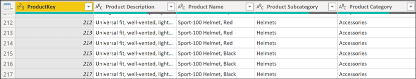
The preview in the Power Query Editor for the Products query should now be similar to that shown in Figure 2.22.

Figure 2.22: Product Query Results

It is not necessary to rename the ProductKey column since this column will be hidden from the reporting layer. In practice, the product dimension would include many more columns. Closing and applying the changes results in only the Products table being loaded into the model.

The denormalized Products table now supports a three-level hierarchy in the Power BI Desktop model to significantly benefit reporting and analysis.

Figure 2.23: Product Hierarchy

How it works

The default join kind for Table.NestedJoin is a left outer join. However, as other join kinds are supported (for example, inner, anti, and full outer), explicitly specifying this parameter in expressions is recommended. Left outer joins are required in the Products table example, as the foreign key columns on DimProduct and DimProductSubcategory both allow null values. Inner joins implemented either via Table.NestedJoin or Table.Join functions are recommended for performance purposes otherwise. Additional details on the joining functions as well as tips on designing inline queries as an alternative to staging queries are covered in the Combining and Merging Queries recipe in this chapter.

When a query joins two tables via a Table.NestedJoin or Table.Join function, a column is added to the first table containing a Table object that contains the joined rows from the second table. This column must be expanded using a Table.ExpandTableColumn function, which generates additional rows as specified by the join operation.

Once all rows are generated by the join and column expansion operations, the specific columns desired in the end result can be specified by the Table.SelectColumns operation; these columns can then be renamed as desired using the Table.RenameColumns function.

There's more...

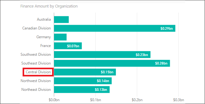
Using Import mode, we can do many things to enhance our queries to aid in report development and display. One such example is that we can add additional columns to provide automatic sorting of an attribute in report visuals. Specifically, suppose that we wish for the United States regional organizations to appear next to one another by default in visualizations. By default, since the Organization column in the DimOrganization table in AdventureWorksDW2019 is a text column, the Central Division (a part of the USA), appears between Canada and France based upon the default alphabetical sorting of text columns. We can modify a simple query that pulls the DimOrganization table to add a numeric sorting column. To see how this works, follow these steps:

1. Using the same Power BI file used for this recipe, open the Power Query Editor, right-click the AdWorksDW query, and select Reference.
2. Choose the DimOrganization table and rename the query to DimOrganization.
3. Open the Advanced Editor window for the DimOrganization query.
4. Add a Table.Sort expression to the import query for the DimOrganization dimension. The columns for the sort should be at the parent or higher level of the hierarchy.
5. Add an expression with the Table.AddIndexColumn function that will add a sequential integer based on the table sort applied in the previous step. The completed query should look something like the following:

   let
       Source = AdWorksDW,
       dbo_DimOrganization = 
           Source{[Schema="dbo",Item="DimOrganization"]}[Data],
       OrgSorted = 
           Table.Sort(
               dbo_DimOrganization,
               {
                   {"ParentOrganizationKey", Order.Ascending},
                   {"CurrencyKey", Order.Ascending}
               }
           ),
       OrgSortIndex = Table.AddIndexColumn(OrgSorted,"OrgSortIndex",1,1) 
   in
       OrgSortIndex
   

6. Finally, with the Ctrl key pressed, select the OrganizationKey, OrganizationName, and OrgSortIndex columns by clicking their column headers. Right-click on the OrgSortIndex column and choose to Remove Other Columns. The preview data should now show as presented in Figure 2.24.

   

Figure 2.24: Modified Organization Dimension Query

With this expression, the table is first sorted by the ParentOrganizationKey column and then by the CurrencyKey column. The new index column starts at the first row of this sorted table with an incremental growth of one per row. The net effect is that all of the US divisions are grouped together at the end of the table.

We can now use this new index column to adjust the default alphanumeric sorting behavior of the OrganizationName column. To see how this works, perform the following steps:

1. Choose Close & Apply to exit Power Query Editor to load the DimOrganization table.
2. In the Data View, select the OrganizationName column.
3. From the Column tools tab, set the Sort by column drop-down to the OrgSortIndex column.

   

   Figure 2.25: Sort By in Data View

4. Finally, right-click on the OrgSortIndex column and select Hide in report view.

Visuals using the OrganizationName column will now sort the values by their parent organization such that the USA organizations appear together (but not alphabetically).

Figure 2.26: Organization automatically sorted

See also

• Dataset modes in the Power BI service: http://bit.ly/30P2HKF
• Data reduction techniques for Import modeling: http://bit.ly/30RsMZI

The application of precise and often complex filter conditions has always been at the heart of business intelligence, and Power BI Desktop supports rich filtering capabilities across its query, data model, and visualization components. In many scenarios, filtering at the query level via the Query Editor and M functions is the optimal choice, as this reduces the workload of both Import and DirectQuery data models and eliminates the need for re-applying the same filter logic across multiple reports or visualizations.

Although the Query Editor graphical interface can be used to configure filtering conditions, this recipe demonstrates M's core filtering functions and the use of M in common multi-condition filter scenarios. The M expression queries constructed in this recipe are intended to highlight some of the most common filtering use cases.

Note that applying data transformations as part of a data warehouse ETL (extract-transform-load) or ELT (extract-load-transform) process is generally preferable to using Power Query (M). BI teams and developers should be careful to avoid creating Power BI datasets that significantly deviate from existing "sources of truth".

The following eight filtering queries will be developed in this recipe:

• United States customers only
• Customers with three or more children
• Customers with null values for either the middle name or title columns
• Customers with first purchase dates between 2012 and 2013
• Customers in management with the female gender or a bachelor's education
• The top 100 customers based on income
• A list of distinct sales territory countries
• Dates less than or equal to the current date and more than ten years prior to the current date

Getting ready

To prepare for this recipe, import the DimCustomer and DimDate tables from the AdventureWorksDW2019 database by doing the following:

1. Open Power BI Desktop and choose Transform data from the ribbon of the Home tab to open the Power Query Editor.
2. Create an Import mode data source query called AdWorksDW. This query should be similar to the following:

   let
       Source = Sql.Database("localhost\MSSQLSERVERDEV", "AdventureWorksDW2019")
   in
       Source
   

3. Isolate this query in a query group called Data Sources.
4. Right-click AdWorksDW and choose Reference.
5. Choose the DimCustomer table and rename the query DimCustomer.
6. Repeat steps 4 and 5 for the DimDate table.
7. Group the dimension queries into a query group called Base Queries.
8. Disable the loading of all queries.
9. For the DimCustomer query, find the DimGeography column. In the column header, click the diverging arrows icon, uncheck (Select All Columns), and then check the box next to CountryRegionCode and DimSalesTerritory before clicking the OK button.

   

   Figure 2.27: Expanding DimGeography to Include CountryRegionCode and DimSalesTerritory

10. Now expand DimGeography.DimSalesTerritory and only select the SalesTerritoryCountry column.
11. Rename the DimGeography.CountryRegionCode column to CountryCode and the DimGeography.DimSalesTerritory.SalesTerritoryCountry column to SalesTerritoryCountry.

For additional details on performing these steps, see the Managing Queries and Data Sources recipe in this chapter.

How to Apply Multiple Functions

To implement this recipe, use the following steps:

1. Right-click the DimCustomer query, choose Reference, and then open the Advanced Editor window for this query. Use the Table.SelectRows function to apply the US query predicate and rename the query United States Customers. The finished query should appear the same as the following:

   let
       Source = DimCustomer,
       USCustomers = Table.SelectRows(Source, each [CountryCode] = "US")
   in
       USCustomers
   

2. Repeat step 1, but this time filter on the TotalChildren column for >= 3 and rename this query Customers w3+ Children:

   let
       Source = DimCustomer,
       ThreePlusChildFamilies = Table.SelectRows(Source, each [TotalChildren] >=3)
   in
       ThreePlusChildFamilies
   

3. Repeat step 1, but this time use the conditional logic operator or to define the filter condition for blank values in the MiddleName or Title columns. Use lowercase literal null to represent blank values. Name this query Missing Titles or Middle Names:

   let
       Source = DimCustomer,
       MissingTitleorMiddleName = 
           Table.SelectRows(
               Source, each [MiddleName] = null or [Title] = null
           )
   in
       MissingTitleorMiddleName
   

4. Repeat step 1, but this time use the #date literal to apply the 2012-2013 filter on the DateFirstPurchase column. Rename this query 2012-2013 First Purchase Customers:

   let
       Source = DimCustomer,
       BetweenDates = 
           Table.SelectRows(
               Source,
               each [DateFirstPurchase] >= #date(2012,01,01) and
                    [DateFirstPurchase] <= #date(2013,12,31)
           )
   in
       BetweenDates
   

5. Repeat step 1, but this time use parentheses to define the filter conditions for an EnglishOccupation of Management, and either the female gender (F), or Bachelors education. The parentheses ensure that the or condition filters are isolated from the filter on Occupation. Rename this query Management and Female or Bachelors:

   let
       Source = DimCustomer,
       MgmtAndFemaleOrBachelors = 
           Table.SelectRows(
               Source,
               each [EnglishOccupation] = "Management" and
               ([Gender] = "F" or [EnglishEducation] = "Bachelors")
           )
   in
       MgmtAndFemaleOrBachelors
   

6. Right-click the United States Customers query, select Reference, and open the Advanced Editor. This time, use the Table.Sort function to order this table by the YearlyIncome column. Finally, use the Table.FirstN function to retrieve the top 100 rows. Rename this query to Top US Customers by Income.

   let
       Source = #"United States Customers",
       SortedByIncome = 
           Table.Sort(
               Source,
               {{"YearlyIncome", Order.Descending}}
           ),
       TopUSIncomeCustomers = Table.FirstN(SortedByIncome,100)
   in
       TopUSIncomeCustomers
   

7. Repeat step 1, but this time use the List.Distinct and List.Sort functions to retrieve a distinct list of values from the SalesTerritoryCountry column. Rename this query Customer Sales Territory List.

   let
       Source = DimCustomer,
       SalesTerritoryCountryList = List.Distinct(Source[SalesTerritoryCountry]),
       OrderedList = List.Sort(SalesTerritoryCountryList,Order.Ascending)
   in
       OrderedList
   

8. Group the queries created thus far into a Customer Filter Queries query group.
9. Create a new query by referencing DimDate and open the Advanced Editor. Use the DateTime.LocalNow, DateTime.Date, and Date.Year functions to retrieve the trailing ten years from the current date. Rename this query Trailing Ten Years from Today and place this query in its own group, Date Filter Queries.

   let
       Source = DimDate,
       TrailingTenYearsFromToday = 
           Table.SelectRows(
               Source,
               each 
                   [FullDateAlternateKey] <= DateTime.Date(DateTime.LocalNow) and
                   [CalendarYear] >= Date.Year(DateTime.LocalNow) - 10
           )
   in
       TrailingTenYearsFromToday
   

How it works

The Table.SelectRows function is the primary table-filtering function in the M language, and is functionally aligned with the FROM and WHERE clauses of SQL. Observe that variable names are used as inputs to M functions, such as the Source line being used as the first parameter to the Table.SelectRows function.

Readers should not be concerned with the each syntax of the Table.SelectRows function. In many languages, this would suggest row-by-row iteration, but when possible, the M engine folds the function into the WHERE clause of the SQL query submitted to the source system.

In the queries United States Customers, Customers w3+ Children, Missing Titles or Middle Names, and Management and Female or Bachelors, notice the various forms of the each selection condition. The syntax supports multiple comparison operators as well as complex logic, including the use of parenthesis to isolate logical tests.

In the 2012-2013 First Purchase Customers query, the #date literal function is used to generate the comparison values. Literals are also available for DateTime (#datetime), Duration (#duration), Time (#time), and DateTimeZone (#datetimezone).

In the Top US Customers by Income query, the Table.Sort function is used to sort the rows by a specified column and sort order. The Table.Sort function also supports multiple columns as per the Importing Data recipe in this chapter. The Table.FirstN function is then used to return 100 rows starting from the very top of the sorted table. In this example, the set returned is not deterministic due to ties in income.

The Customer Sales Territory List query returns a list instead of a table. This is evident from the different icon present in the Queries pane for this query versus the others. Lists are distinct from tables in M, and one must use a different set of functions when dealing with lists rather than tables. A list of distinct values can be used in multiple ways, such as a dynamic source of available input values to parameters.

Finally, in the Trailing 10 Yrs from Today query, the current date and year are retrieved from the DateTime.LocalNow function and then compared to columns from the date dimension with these values.

There's more...

With simple filtering conditions, as well as in proof-of-concept projects, using the UI to develop filter conditions may be helpful to expedite query development. However, the developer should review the M expressions generated by these interfaces, as they are only based on the previews of data available at design time, and logical filter assumptions can be made under certain conditions.

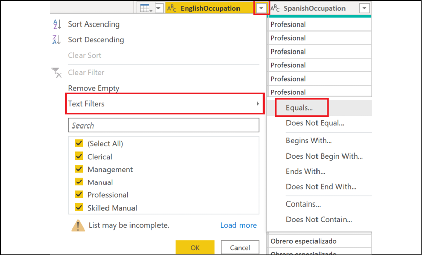
To access the Filter Rows dialog, click on the drop-down button in a column header and then choose the Text Filters option, before specifying a starting filtering condition.

Figure 2.28: Accessing the Filter Rows dialog

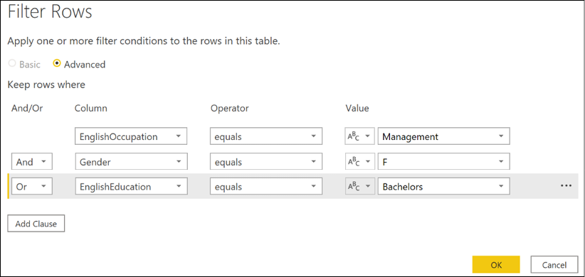
The Basic option of the Filter Rows dialog only allows you to work with the currently selected column. However, by clicking on the Advanced radio button, you can work with any column in the table.

Figure 2.29: Advanced Filter Rows dialog in the Query Editor

Despite this, even the Advanced version of the Filter Rows dialog does not provide the ability to group logical filtering criteria. While the dialog in Figure 2.29 looks like it recreates the query for Management and Female or Bachelors, the generated M code does not include the parenthesis that groups the Gender and EnglishEducation clauses. Thus, the code generated would have to be edited manually in the Advanced Editor to return the same results as the original Management and Female or Bachelors query. The M code generated by the Filter Rows dialog shown in Figure 2.29 generates the following code:

        Table.SelectRows(
            Source, 
            each 
                [EnglishOccupation] = "Management" and 
                [Gender] = "F" or 
                [EnglishEducation] = "Bachelors"
        )

See also

• Table.SelectRows: http://bit.ly/3bSkEyj
• Table.Sort: http://bit.ly/3qPaeUo
• Table.FirstN: http://bit.ly/3ttb0In
• List.Distinct: http://bit.ly/3lnCqwq
• List.Sort: http://bit.ly/30QLEb1
• 10 Common Mistakes You Do In #PowerBI #PowerQuery – Pitfall #3: http://bit.ly/2nLX6QW

The columns selected in data retrieval queries impact the performance and scalability of both import and DirectQuery data models. For Import models, the resources required by the refresh process and the size of the compressed data model are directly impacted by column selection. Specifically, the cardinality of columns drives their individual memory footprint and memory per column. This correlates closely to query duration when these columns are referenced in measures and report visuals. For DirectQuery models, the performance of report queries is directly affected. Regardless of the model type, the way in which this selection is implemented also impacts the robustness of the retrieval process. Additionally, the names assigned to columns (or accepted from the source) directly impact the Q&A or natural language query experience.

This recipe identifies columns to include or exclude in a data retrieval process and demonstrates how to select those columns as well as the impact of those choices on the data model. In addition, examples are provided for applying user-friendly names and other considerations for choosing to retrieve or eliminate columns of data for retrieval.

Getting ready

To get ready for this recipe, import the DimCustomer table from the AdventureWorksDW2019 database by doing the following:

1. Open Power BI Desktop and choose Transform data from the ribbon of the Home tab to open the Power Query Editor.
2. Create an Import mode data source query called AdWorksDW. This query should be similar to the following:

   let
       Source = Sql.Database("localhost\MSSQLSERVERDEV", "AdventureWorksDW2019")
   in
       Source
   

3. Isolate this query in a query group called Data Sources.
4. Right-click AdWorksDW and choose Reference.
5. Select the DimCustomer table in the data preview area and rename this query DimCustomer.

For additional details on performing these steps, see the Managing Queries and Data Sources recipe in this chapter.

How to Select and Rename Columns

To implement this recipe, use the following steps in Advanced Editor:

1. Create a name column from the first and last names via the Table.AddColumn function.

       CustomerNameAdd = 
           Table.AddColumn(
               dbo_DimCustomer, "Customer Name",
               each [FirstName] & " " & [LastName],
               type text
           )
   

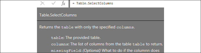
2. Use the Table.SelectColumns function to select 10 of the 30 available columns now available in the DimCustomer table.

       SelectCustCols = 
           Table.SelectColumns(CustomerNameAdd,
               {
                   "CustomerKey", "Customer Name", "Annual Income", 
                   "Customer Gender", "Customer Education", "MaritalStatus", 
                   "Customer Phone Number", "CommuteDistance", "AddressLine1", 
                   "TotalChildren"
               }, MissingField.UseNull
           )
   

   Note that some of the column names specified do not actually exist. This is on purpose and will be fixed in the next step. But note that instead of generating an error, null values are displayed for those columns.

   

Figure 30: Non-existent columns return null instead of error

Use the Table.RenameColumns function to apply intuitive names for users and benefit the Q&A engine for natural language queries. Insert this statement above your SelectCustCols statement and adjust as appropriate. The full query should now be similar to the following:

let
    Source = AdWorksDW,
    dbo_DimCustomer = Source{[Schema="dbo",Item="DimCustomer"]}[Data],
    CustomerNameAdd = 
        Table.AddColumn(
            dbo_DimCustomer, "Customer Name",
            each [FirstName] & " " & [LastName],
            type text
        ),
    #"Renamed Columns" = 
        Table.RenameColumns(CustomerNameAdd,
            {
                {"YearlyIncome", "Annual Income"}, 
                {"Gender", "Customer Gender"},
                {"EnglishEducation", "Customer Education"},
                {"Phone", "Customer Phone Number"}
            }
        ),
    SelectCustCols = 
        Table.SelectColumns(#"Renamed Columns",
            {
                "CustomerKey", "Customer Name", "Annual Income", 
                "Customer Gender", "Customer Education", "MaritalStatus", 
                "Customer Phone Number", "CommuteDistance", "AddressLine1", 
                "TotalChildren"
            }, MissingField.UseNull
        )
in
    SelectCustCols

How it works

The Table.AddColumn function concatenates the FirstName and LastName columns and includes an optional final parameter that specifies the column type as text.

The Table.SelectColumns function specifies the columns to retrieve from the data source. Columns not specified are excluded from retrieval.

A different method of accomplishing this same effect would be to use the Table.RemoveColumns function. However, in this case, 20 columns would need to be removed versus explicitly defining 10 columns to keep. To avoid query failure if one of the source columns changes or is missing, it is better to specify and name 10 than 20 columns. Query resilience can further be improved by using the optional parameter for Table.SelectColumns, MissingField.UseNull. Using this parameter, if the column selected is not available, the query still succeeds and simply inserts null values for this column for all rows.

Another advantage of using the Table.SelectColumns function is that columns can be reordered as selected columns are retrieved and presented in the order specified. This can be helpful for the query design process and avoids the need for an additional expression with a Table.ReorderColumns function. The initial column order of a query loaded to the data model is respected in the Data view. However, the field list exposed in the Fields pane in both the Report and Data views of Power BI Desktop is automatically alphabetized.

For import data models, you might consider removing a column that represents a simple expression of other columns from the same table. For example, if the Extended Amount column is equal to the multiplication of the Unit Price and Order Quantity columns, you can choose to only import these latter two columns. A DAX measure can instead compute the Extended Amount value. This might be done to keep model sizes smaller. This technique is not recommended for DirectQuery models, however.

Use the Table.RenameColumns function to rename columns in order to remove any source system indicators, add a space between words for non-key columns, and apply dimension-specific names such as Customer Gender rather than Gender. The Table.RenameColumns function also offers the MissingField.UseNull option.

There's more...

Import models are internally stored in a columnar compressed format. The compressed data for each column contributes to the total disk size of the file. The primary factor of data size is a column's cardinality. Columns with many unique values do not compress well and thus consume more space. Eliminating columns with high cardinality can reduce the size of the data model and thus the overall file size of a PBIX file. However, it is the size of the individual columns being accessed by queries that, among other factors, drives query performance for import models.

See also

• Table.SelectColumns: http://bit.ly/38Qk7Lt
• Table.RenameColumns: http://bit.ly/3rTVfd4
• Table.RemoveColumns: http://bit.ly/3cJju7p
• Table.ReorderColumns: http://bit.ly/3cEoOJg
• Table.AddColumn: http://bit.ly/3vGJZ6b
• Power BI Documentation on preparing data for Q&A: http://bit.ly/2nBLAGc

The transformations applied within Power BI's M queries serve to protect the integrity of the data model and to support enhanced analysis and visualization. The specific transformations to implement varies based on data quality, integration needs, and the goals of the overall solution. However, at a minimum, developers should look to protect the integrity of the model's relationships and to simplify the user experience via denormalization and standardization. Additionally, developers should check with owners of the data source to determine whether certain required transformations can be implemented in the source, or perhaps made available via SQL view objects such that Power Query (M) expressions are not necessary.

This recipe demonstrates how to protect a model from duplicate values within the source data that can prevent forming proper relationships within the data model, which may even result in query failures. While a simple scenario is used, this recipe demonstrates scenarios you may run into while attempting to merge multiple data sources and eliminating duplicates.

Getting ready

To prepare, start by importing the DimProduct and FactResellerSales tables from the AdventureWorksDW2019 database by doing the following:

1. Open Power BI Desktop and choose Transform data from the ribbon of the Home tab to open the Power Query Editor.
2. Create an Import mode data source query called AdWorksDW. This query should be similar to the following:

   let
       Source = Sql.Database("localhost\MSSQLSERVERDEV", "AdventureWorksDW2019")
   in
       Source
   

3. Isolate this query in a query group called Data Sources.
4. Right-click AdWorksDW and choose Reference, select the DimProduct table in the data preview area, and rename this query DimProduct. Right-click the EnglishProductName column and select Remove Other Columns.
5. Repeat the previous step, but this time choose FactResellerSales. Expand the DimProduct column and only choose EnglishProductName. Rename this column to EnglishProductName.
6. Drag the DimProduct and FactResellerSales queries into the Other Queries group and apply the queries to the data model.
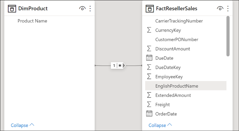
7. In the Model view of Power BI Desktop, attempt to form a relationship between the tables using the EnglishProductName columns from both tables. Note the warning that is displayed.

   

Figure 2.31: Many-Many relationship cardinality warning

For additional details on performing these steps, see the Managing Queries and Data Sources recipe in this chapter.

How to Transform and Cleanse Data

We wish to remove duplicates from the EnglishProductName column in our DimProduct query. To implement this recipe, use the following steps:

1. Remove any leading and trailing empty spaces in the EnglishProductName column with a Text.Trim function.
2. Create a duplicate column of the EnglishProductName key column with the Table.DuplicateColumn function and name this new column Product Name.
3. Add an expression to force uppercase on the EnglishProductName column via the Table.TransformColumns function. This new expression must be applied before the duplicate removal expressions are applied.
4. Add an expression to the DimProduct query with the Table.Distinct function to remove duplicate rows.
5. Add another Table.Distinct expression to specifically remove duplicate values from the EnglishProductName column.
6. Drop the capitalized EnglishProductName column via Table.RemoveColumns.

   The final query should resemble the following:

   let
       Source = AdWorksDW,
       dbo_DimProduct = Source{[Schema="dbo",Item="DimProduct"]}[Data],
       RemoveColumns = Table.SelectColumns(dbo_DimProduct,{"EnglishProductName"}),
       TrimText = 
           Table.TransformColumns(
               RemoveColumns,{"EnglishProductName",Text.Trim}
           ),
       DuplicateKey = 
           Table.DuplicateColumn(
               TrimText,"EnglishProductName","Product Name"
           ),
       UpperCase = 
           Table.TransformColumns(
               DuplicateKey,{{"EnglishProductName", Text.Upper}}
           ),
       DistinctProductRows = Table.Distinct(UpperCase),
       DistinctProductNames = 
           Table.Distinct(
               DistinctProductRows, {"EnglishProductName"}
           ),
       RemoveEnglishProductName = 
           Table.RemoveColumns(
               DistinctProductNames,"EnglishProductName"
           )
   in
       RemoveEnglishProductName
   

How it works

In the TrimText expression, the Trim.Text function removes white space from the beginning and end of a column. Different amounts of empty space make those rows distinct within the query engine, but not necessarily distinct within the model. Therefore, it is always a good idea to use Trim.Text first and then remove duplicate rows and values.

In the next expression, DuplicateKey, the Table.DuplicateColumn function is used to duplicate the column where we will be removing duplicate values. We give this new column the name that we desire for our final column. This is done because we will need to transform the values in the column we are removing duplicates from, in order to account for mixed cases such as "Fender Set" and "Fender set". Thus, we wish to preserve the original values and casing by using this duplicate column.

In order to eliminate mixed casing issues, the UpperCase expression changes all values in the EnglishProductName column to uppercase using the Table.TransformColumns function, and specifying Text.Upper. The M engine considers mixed casing values unique, but the data model engine does not.

The next two expressions, DistinctProductRows and DistinctProductNames, simply demonstrate two different methods of using the Table.Distinct function. The first, DistinctProductRows, eliminates rows where the entire row (all column values) are identical. The second version looks only at the values in a single column when determining whether or not the row is a duplicate.

At this point, the query is now resilient to duplicate values and rows, mixed cases, and spaces. However, the EnglishProductName column is now in the uppercase format. Since we preserved a copy of the original values and casing in our Product Name column, we can simply drop the EnglishProductName column using the Table.RemoveColumns function.

We can now form a one-to-many relationship between our DimProduct and FactResellerSales tables.

Figure 2.32: Simple one-to-many relationship model

There's more...

To support troubleshooting, create a query that accesses the same source table and retrieves the values from the EnglishProductName column with more than one row.

let
    Source = AdWorksDW,
    dbo_DimProduct = Source{[Schema="dbo",Item="DimProduct"]}[Data],
    RemoveColumns = Table.SelectColumns(dbo_DimProduct,{"EnglishProductName"}),
    TrimText = 
        Table.TransformColumns(
            RemoveColumns,{"EnglishProductName",Text.Trim}
        ),
    UpperCase = 
        Table.TransformColumns(
            TrimText,{{"EnglishProductName", Text.Upper}}
        ),
    GroupedRows = 
        Table.Group(
            UpperCase, {"EnglishProductName"},
            {{"Rows", each Table.RowCount(_), Int64.Type}}
        ),
    Duplicates = Table.SelectRows(GroupedRows, each [Rows] > 1)
in
    Duplicates

The EnglishProductName column is selected, trimmed, converted to uppercase, grouped, and then filtered to always retrieve any duplicate key values. Disable the loading of this query, as the query would only exist for troubleshooting purposes.

See also

• Table.SelectColumns: http://bit.ly/38Qk7Lt
• Table.RemoveColumns: http://bit.ly/3cJju7p
• Table.TransformColumns: http://bit.ly/3tsdxm2
• Table.DuplicateColumn: http://bit.ly/3cIF63X
• Table.Distinct: http://bit.ly/38V8mmN
• Text.Trim: http://bit.ly/3eUmAZ0
• Text.Upper: http://bit.ly/3vFW2R6
• M functions reference for text: http://bit.ly/2nUYjnw

Business users often extend the outputs of existing reports and data models with additional columns to help them analyze and present data. The logic of these columns is generally implemented through Excel formulas or as calculated DAX columns. A superior solution, particularly if the logic cannot quickly be migrated to a data warehouse or IT resource, is to create the columns via the Power Query Editor and M language.

Developing custom columns can also significantly enhance the ease of use and analytical power of data models and the visualizations they support. In this recipe, columns are created to apply a custom naming format and simplify the analysis of a customer dimension via existing columns.

Getting ready

To get ready for this recipe, import the DimCustomer table from the AdventureWorksDW2019 database by doing the following:

1. Open Power BI Desktop and choose Transform data from the ribbon of the Home tab to open the Power Query Editor.
2. Create an Import mode data source query called AdWorksDW. This query should be similar to the following:

   let
       Source = Sql.Database("localhost\MSSQLSERVERDEV", "AdventureWorksDW2019")
   in
       Source
   

3. Isolate this query in a query group called Data Sources.
4. Right-click AdWorksDW and choose Reference, select the DimCustomer table in the data preview area, and rename this query DimCustomer.

For additional details on performing these steps, see the Managing Queries and Data Sources recipe in this chapter.

How to Create Custom Columns

To implement this recipe, perform the following steps:

1. Use Table.SelectColumns to retrieve the required source columns from the DimCustomer table, FirstName, LastName, MiddleName, Title and BirthDate.

   let
       Source = AdWorksDW,
       dbo_DimCustomer = Source{[Schema="dbo",Item="DimCustomer"]}[Data],
       SelectColumns = 
           Table.SelectColumns(dbo_DimCustomer,
               {"FirstName", "LastName", "MiddleName", "Title", "BirthDate"}
           )
   in
       SelectColumns
   

2. Write a Table.AddColumns function with an if...then expression that accounts for the different scenarios given a target format of Mr. John A. Doe:

       NameFormatTble = 
           Table.AddColumn(
               SelectColumns,"Formatted Name", each
                   if [Title] = null and [MiddleName] = null 
                       then [FirstName] & " " & [LastName] 
                   else if [Title] = null 
                       then [FirstName] & " " & Text.Range([MiddleName],0,1) 
                               & ". " & [LastName]
                   else
                       [Title] & " " & [FirstName] & " " 
                           & Text.Range([MiddleName],0,1) & ". " & [LastName]
           )
   

3. Add variables that allow the expression to support the comparison between the current system date and the BirthDate column.

   let
       CurrentDate = DateTime.Date(DateTime.LocalNow()),
       CurrentYear = Date.Year(CurrentDate),
       CurrentMonth = Date.Month(CurrentDate),
       CurrentDay = Date.Day(CurrentDate),
       Source = AdWorksDW,
   

4. Use the Table.AddColumn function to create Customer Year, Customer Month, and Customer Day columns based upon the BirthDate column.

       AddCustomerYear = 
           Table.AddColumn(
               NameFormatTble, "Customer Year", each Date.Year([BirthDate]),
               Int64.Type
           ),
       AddCustomerMonth = 
           Table.AddColumn(
               AddCustomerYear, "Customer Month", each Date.Month([BirthDate]),
               Int64.Type
           ),
       AddCustomerDay = 
           Table.AddColumn(
               AddCustomerMonth, "Customer Day", each Date.Day([BirthDate]),
               Int64.Type
           )
   

5. Add an Age column via an if...then expression.

       CustomerAge = 
           Table.AddColumn(
               AddCustomerDay,"Customer Age", each
               if [Customer Month] < CurrentMonth 
                   then CurrentYear - [Customer Year]
               else if [Customer Month] > CurrentMonth 
                   then CurrentYear - [Customer Year] - 1
               else if [Customer Day] < CurrentDay 
                   then CurrentYear - [Customer Year]
               else CurrentYear - [Customer Year] - 1
           )
   

6. Add a Customer Age Segment column via the column computed in step 4.

       CustomerSegment = 
           Table.AddColumn(
               CustomerAge, "Customer Age Segment", each
               if [Customer Age] < 30 then "Less than 30"
               else if [Customer Age] < 40 then "30 to 39"
               else if [Customer Age] < 50 then "40 to 49"
               else if [Customer Age] < 60 then "50 to 59"
               else "60 or Older"
           )
   

How it works

In the NameFormatTble expression the Table.AddColumn function is used, coupled with an if...then expression. M is a case-sensitive language, so writing IF instead of if or Table.Addcolumn instead of Table.AddColumn will return an error. if...then expressions follow the following structure:

if <condition1> then <result1> else <result2>

All three inputs (condition1, result1, and result2) accept M expressions. if expressions can be nested together with the following structure:

if <condition1> then <result1> else if <condition2> then <result2> else <result3>

The equivalent of a SQL CASE expression is not available in M. However, the order of conditions specified in if...then expressions drives the evaluation process. Multiple conditions could be true but the second and later conditions will be discarded and not evaluated. If the value produced by the if condition is not a logical value, an error is raised.

The three if...then conditions in the NameFormatTble expression account for all scenarios to return the formatted name, since the query must account for nulls in the Middle Name and Title columns, as well as different values in the Middle Name column. Text.Range is used to extract the first character of the middle name.

For the variables CurrentDate, CurrentYear, CurrentMonth, and CurrentDay, the DateTime.LocalNow function is used as the source for the current date; it is then used for year, month, and day.

For the AddCustomerYear, AddCustomerMonth, and AddCustomerDay expressions, the Int64.Type value is passed to the optional type parameter of Table.AddColumn to set the new columns as whole numbers.

For the CustomerAge and CustomerSegment expressions, nested if…then expressions are used. This method is used because, currently, the equivalent of a DATEDIFF function (T-SQL, DAX) with date intervals like Year, Month, Week, and so on, are not available in M. A Duration.Days function can be used for day intervals and additional duration functions are available for hour, minute, and second intervals.

The CustomerAge expression compares the CurrentMonth and CurrentDay variables against the values of the customer columns created in the AddCustomerMonth and AddCustomerDay expressions in order to compute the age of the customer using the CurrentYear variable and the column created by the AddCustomerYear expression. The column created by the CustomerAge column is then used in the CustomerSegement expression to derive the age segmentation column. The new custom columns can be used to support various visualizations based upon the ages and segmentation of customers.

There's more...

The Power Query Editor provides graphical user interfaces for adding columns. These interfaces provide mechanisms for adding columns that are an alternative to writing out the code manually. In essence, the M code for the added columns is generated as an output from these interfaces.

One such interface is the Column From Examples feature, which allows users to simply type examples of a desired column's output. The engine determines which M functions and series of steps to add to the query that return results consistent with the examples provided. To explore this feature, follow these steps:

1. Create a new query referencing the AdWorksDW query.
2. Select the DimCustomer table.
3. Select the Title, FirstName, MiddleName, LastName, and BirthDate columns and remove all other columns.
4. Select the Add Column tab and then choose the Column From Examples button in the ribbon.

   

   Figure 2.33: Column From Examples feature

5. Type the customer's FirstName, MiddleName, and LastName values into the first row and hit the Enter key. Notice that the rest of the rows are automatically calculated based upon this first row.

   

   Figure 2.34: Column From Examples interface

6. Click the OK button to accept the transformation.

Another interface for adding columns is the Condition Column feature. This feature provides a method of creating conditional columns as an alternative to writing out the if...then expressions. To see how this feature operates, follow these steps:

1. Select the Add Column tab and then select Conditional Column from the ribbon.

   

   Figure 2.35: Conditional Column feature

2. Fill in the fields on the Add Conditional Column dialog, using the Add Clause button to add additional else if statements; click the OK button to exit the dialog and create the new column.

   

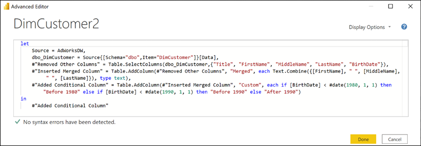
Figure 2.36: Add Conditional Column dialog

Any column from the table can be referenced, and multiple created steps can be moved up or down the order of evaluation using the ellipses (…). Open the Advanced Editor to inspect the code created.

Figure 2.37: Added conditional column M code

See also

• Table.AddColumn: http://bit.ly/3vGJZ6b
• Table.SelectColumns: http://bit.ly/38Qk7Lt
• DateTime functions: http://bit.ly/3tPtKlJ
• Add Column From examples: http://bit.ly/3eWTLv6

The full power of Power BI's querying capabilities is in the integration of distinct queries representing different data sources via its merge and append transformations. Retrieval processes that consolidate files from multiple network locations or integrate data from multiple data sources can be developed efficiently and securely. Additionally, the same join types and data transformation patterns SQL and ETL developers are familiar with can be achieved with the M language. This recipe provides examples of combining sources into a single query and leveraging the table join functions of M to support common transformation scenarios.

Getting ready

To follow along with this recipe, you can use the Merge Queries and Append Queries icons on the Home tab of the Power Query Editor to generate the join expressions used in this recipe. However, as joining queries is fundamental to the retrieval process, it is recommended to learn how to use the Table.Join, Table.NestedJoin, and Table.Combine functions.

To get ready for this recipe, import the DimCustomer and FactCallCenter tables from the AdventureWorksDW2019 database by doing the following:

1. Open Power BI Desktop and choose Transform data from the ribbon of the Home tab to open the Power Query Editor.
2. Create an Import mode data source query called AdWorksDW. This query should be similar to the following:

   let
       Source = Sql.Database("localhost\MSSQLSERVERDEV", "AdventureWorksDW2019")
   in
       Source
   

3. Isolate this query in a query group called Data Sources.
4. Right-click AdWorksDW and choose Reference, select the DimEmployee table in the data preview area, and rename this query DimEmployee.
5. Repeat step 4 but choose the FactInternetSales table and name this query Sales2011. Filter the OrderDate column to be between January 1, 2011 and December 31, 2011.

   Let
       Source = AdWorksDW,
       dbo_FactInternetSales = Source{[Schema="dbo",Item="FactInternetSales"]}[Data],
       #"Filtered Rows" = 
           Table.SelectRows(
               dbo_FactInternetSales, each 
                   [OrderDate] >= #datetime(2011, 1, 1, 0, 0, 0) and 
                   [OrderDate] <= #datetime(2011, 12, 31, 0, 0, 0))
   in
       #"Filtered Rows"
   

6. Right-click the Sales2011 query and choose Duplicate. Name this query Sales2012. Edit the Table.SelectRows expression to filter dates between January 1, 2012 and December 31, 2012.
7. Repeat step 6, naming this new query Sales2013 and filtering for dates between January 1, 2013 and December 31, 2013.

For additional details on performing these steps, see the Managing Queries and Data Sources recipe in this chapter.

How to Combine Queries

The goal of this example is to produce an integrated table based on three "Sales" queries. While in this example the three queries come from the same data source, it is important to realize that the three queries could point to completely different data sources, such as three text files or even a text file, an Excel spreadsheet, and a SQL database. What is important is that the three queries have the same column names and number of columns. To implement this recipe, perform the following steps:

1. Move the Sales2011, Sales2012, and Sales2013 queries to a new query group called Staging Queries.
2. Disable the load for the Sales2011, Sales2012, and Sales2013 queries.
3. Create a new Blank query in the Other Queries group and call this query FactInternetSales2011to2012.
4. Open the FactInternetSales2011to2012 query in Advanced Editor.
5. Use the Table.Combine (or Append Queries feature in the ribbon) function to return a single table based on the rows of the Sales2011, Sales2012, and Sales2013 queries.

   Let
       Source = Table.Combine( {Sales2011, Sales2012, Sales2013} )
   in
       Source
   

6. Move the DimEmployees query to the Staging Queries group and disable loading.
7. Duplicate the DimEmployees query and call this new query Managers.
8. Disable loading for the Managers query.
9. Open the Managers query in the Advanced Editor.
10. Add a Manager Name column using the Table.AddColumn function.

        ManagerName = 
            Table.AddColumn(
                dbo_DimEmployee,
                "Manager Name", each [FirstName] & " " & [LastName]
            )
    

11. Select only the EmployeeKey, Manager Name, and Title columns using the Table.SelectColumns function.

        SelectCols = 
            Table.SelectColumns(
                ManagerName, 
                { "EmployeeKey", "Manager Name", "Title" }
            )
    

12. Create a new Blank query in the Other Queries group and call this query Employees.
13. Open the Employees query in Advanced Editor.
14. Join the Managers query and DimEmployee query using the Table.NestedJoin function or the Merge Queries feature in the ribbon.

    Let
        Source = 
            Table.NestedJoin(
                DimEmployee, "ParentEmployeeKey", Managers, "EmployeeKey",
                "ManagerColumn", JoinKind.LeftOuter
            )
    in
        Source
    

15. Use the Table.ExpandTableColumn function to add the Manager Name and Manager Title columns.

        ManagerColumns = 
            Table.ExpandTableColumn(
                Source, "ManagerColumn",
                { "Manager Name", "Title" },
                { "Manager Name", "Manager Title" }
            )
    

16. Add an Employee Name column.

        EmployeeName = 
            Table.AddColumn(
                ManagerColumns,
                "Employee Name", each [FirstName] & " " & [LastName]
            )
    

17. Rename the Title column to Employee Title.

        RenameTitle = 
            Table.RenameColumns(
                EmployeeName,
                { "Title", "Employee Title" }
            )
    

18. Select the EmployeeKey, Employee Name, Employee Title, Manager Name, and Manager Title columns.

        SelectCols =
            Table.SelectColumns(
                RenameTitle,
                { 
                    "EmployeeKey", "Employee Name", "Employee Title",
                    "Manager Name", "Manager Title"
                }
            )
    

How it works

For the FactInternetSales2011to2013 query, only a single expression is required using the Table.Combine function. No other expressions are necessary in this example given that the staging queries have identical column names and the same number of columns. The Table.Combine function performs an append operation and does not remove duplicate rows similar to a SQL UNION statement.

Any columns which are unique to one of the input tables in a Table.Combine function will be added to the result set with null values for the rows from the other tables. Depending on the scenario, the developer could apply the Table.Distinct function to avoid any duplicate rows from reaching the data model.

The Employees query references the DimEmployees query as the left table in a Table.NestedJoin function, and is joined to the Managers query via a left outer join. The left join is required to retain all employee rows in this scenario, as the DimEmployees table includes one employee that does not have a parent employee key, the Chief Executive Officer.

The join is performed on the ParentEmployeeKey column in the DimEmployees query to the EmployeeKey column in the Managers query. After this step, all of the rows from the matching Managers table are stored within the row as a Table object in the column ManagerColumn. When expanding the ManagerColumn column using the Table.ExpandTableColumn function, the Manager Name column can retain the same name, but the Title column is renamed to Manager Title in order to avoid conflicting with the Title column in the DimEmployees query.

In implementing the table joins, you can choose to use the Table.Join and Table.NestedJoin functions. All six join types—inner, left outer, right outer, full outer, left anti, and right anti—are supported by both functions. The Table.NestedJoin function enters the results of the join (the right or second table) into a new column of table values and will use local resources to execute the join operation, unless the Table.ExpandTableColumn function is used to replace this new column with columns from the right table. A left outer join type is the default if the JoinKind parameter is not specified. For performance reasons, Table.NestedJoin should not be used without a Table.ExpandTableColumn function removing the column of tables.

Conversely, the Table.Join function automatically expands the left table with the columns from the right table input (a flat join) and defaults to an inner join if the JoinKind parameter is not specified. The Table.Join function gets folded to the source without any additional functions but requires that there are no matching column names between the joined tables for a JoinKind other than inner join. For inner joins, the matching column names from both tables must be specified in the join key parameters. A Table.SelectColumns function is required to exclude any columns from the right table added with the join.

Whether implemented via Table.NestedJoin or Table.Join, developers should look to use inner joins if the source tables have referential integrity, such as with foreign key constraints and whether this meets requirements. For joins against larger tables, developers should confirm that query folding is occurring and can evaluate the different query plans generated by alternative retrieval designs in terms of performance.

Note that the two rows for Rob Walters are due to a Slowly Changing Dimension (SCD) Type 2 process applied in the source database. For more information on SCDs, refer to this Wikipedia article: https://bit.ly/3yIQeI5.

There's more...

Rather than creating separate lookup/join staging queries, it is possible to consolidate these expressions into a single let…in M expression. For example, the following single query returns the exact same results as the Sales2011, Sales2012, Sales2013, and FactInternetSales2011to2013 queries:

let
    Source = AdWorksDW,
    Sales = Source{[Sche"a=""bo",It"m="FactInternetSa"es"]}[Data],
    Sales2011Rows = 
        Table.SelectRows(
            Sales, each 
                [OrderDate] >= #datetime(2011, 1, 1, 0, 0, 0) and 
                [OrderDate] <= #datetime(2011, 12, 31, 0, 0, 0)
        ),
    Sales2012Rows = 
        Table.SelectRows(
            Sales, each 
                [OrderDate] >= #datetime(2012, 1, 1, 0, 0, 0) and 
                [OrderDate] <= #datetime(2012, 12, 31, 0, 0, 0)
        ),
    Sales2013Rows = 
        Table.SelectRows(
            Sales, each 
                [OrderDate] >= #datetime(2013, 1, 1, 0, 0, 0) and 
                [OrderDate] <= #datetime(2013, 12, 31, 0, 0, 0)
        ),
    Append = Table.Combine( {Sales2011Rows, Sales2012Rows, Sales2013Rows} )
in
    Append

Inline query approaches are helpful in limiting the volume of queries, but you lose the management benefits provided by group folders and the Query Dependencies view. The graphical support makes it easier to explain and quickly troubleshoot a data retrieval process over a single but complex M expression. Staging queries are recommended for all but the most trivial projects and retrieval processes. Staging queries should generally never be loaded to the data model, as staging tables could both confuse the user and would require the data model to use additional resources to process and store the additional data.

Similarly, merge queries can also be combined into a single query. The following table breaks down the six different join types that can be specified in both the Table.NestedJoin and Table.Join functions. Both the Parameter and Parameter Value can be used, though the recipes in this book use Parameter as this makes the expressions easier to follow.

Table 2.3: Power Query (M) join types, parameters, and parameter values

One final note is that, for data source files with the same structure stored in the same network directory folder, Power BI offers the Combine Binaries transformation, which can be used with text, CSV, Excel, JSON, and other file formats. This feature can be used when creating a Folder query. The Combine Binaries feature automatically creates an example query and a function linked to this query, such that any required modification to the source files can be applied to all files, and the source location of the files can be easily revised.

See also

• Table.Combine: http://bit.ly/3c6L2o0
• Table.NestedJoin: http://bit.ly/30ZO3jZ
• Table.Join: http://bit.ly/3lxMRh7
• Table.ExpandTableColumn: http://bit.ly/3eY6u0z
• Table.AddColumn: http://bit.ly/3vGJZ6b
• Table.SelectColumns: http://bit.ly/38Qk7Lt
• Table.RenameColumns: http://bit.ly/3rTVfd4
• M table function reference: http://bit.ly/2oj0k0I
• Combining binaries in Power BI Desktop: http://bit.ly/2oL2nM4

Setting the data types of columns in Power BI Desktop is usually the final step of data retrieval queries, and has great implications for all layers of the solution, including data refresh, data modeling, and visualization. Choosing appropriate data types reduces the risk of refresh failures, ensures consistent report results, and provides analytical flexibility to the data model and visualization layers.

This recipe demonstrates how to choose and define data types to load to Power BI Desktop. Additional details on data types and the implications of data types for Power BI development are contained in the sections following these examples.

Getting ready

In preparation for this recipe, import the FactCallCenter table from the AdventureWorksDW2019 database by doing the following:

1. Open Power BI Desktop and choose Transform data from the ribbon of the Home tab to open the Power Query Editor.
2. Create an Import mode data source query called AdWorksDW. This query should be similar to the following:

   let
       Source = Sql.Database("localhost\MSSQLSERVERDEV", "AdventureWorksDW2019")
   in
       Source
   

3. Isolate this query in a query group called Data Sources.
4. Right-click AdWorksDW and choose Reference, select the FactFinance table in the data preview area, and rename this query FactFinance.
5. Move the FactFinance query to the Other Queries group.

For additional details on performing these steps, see the Managing Queries and Data Sources recipe in this chapter.

How to Select Column Data Types

To implement this recipe, perform the following steps:

1. Use the Table.TransformColumnTypes function to revise the type of the numeric integer FinanceKey column to text. Note that the column header for the FinanceKey column is initially prefaced with a 123 icon and changes to an ABC icon. Also, note that the row values are initially left justified and italicized and after transformation to text are aligned to the right and not italicized.

   let
       Source = AdWorksDW,
       dbo_FactFinance = Source{[Schema="dbo",Item="FactFinance"]}[Data],
       FinanceKeyText = 
           Table.TransformColumnTypes(
               dbo_FactFinance, {{"FinanceKey", Text.Type}}
           )
   in
       FinanceKeyText
   

2. Add a numeric column from a source column stored as text using the Number.FromText and Table.AddColumn functions.

       FinanceKeyNum = 
           Table.AddColumn(
               FinanceKeyText, "FinanceKeyNum",
               each Number.FromText([FinanceKey]),Int64.Type
           )
   

3. Change the fixed decimal Amount column to currency using the Table.TransformColumnTypes function. Note that the column header icon changes from 1.2 initially to a dollar sign, $.

       Currency = 
           Table.TransformColumnTypes(
               FinanceKeyNum,{{"Amount", Currency.Type}}
           )
   

How it works

For the FinanceKeyText expression, the Table.TransformColumnTypes function takes two parameters. The first parameter is the table to operate upon; the second is a list of list pairs that include the column name to transform and then the transformation data type. Multiple pairs can be included in the form:

{ { "Column1", type }, { "Column2", type } }

Additional valid values for the type parameter include the following:

• Currency.Type sets the column as a Fixed Decimal Number to two decimal places.
• Decimal.Type or type number sets the new column as a Decimal Number.
• Percentage.Type sets the column as a Percentage data type. Unlike Whole Number, Fixed Decimal Number, and Decimal Number, this type does not have a corresponding type in the data model. When loaded to the data model, the Percentage data type is represented as a Decimal Number type.
• Text.Type or type text sets the column to a Text data type.
• Date.Type or type date sets the column to a Date data type.
• DateTime.Type or type datetime sets the column to a Date Time data type.
• DateTimeZone.Type or type datetimezone sets the column to a Date/Time/Timezone data type.
• Time.Type or type time sets the column to a Time data type.
• Duration.Type or type duration sets the column to a Duration data type.
• Logical.Type or type logical sets the column to a True/False data type.
• Binary.Type or type binary sets the column to a Binary data type.

Like all M expressions, data type declarations are case-sensitive.

For the FinanceKeyNum expression, the type parameter for the Table.AddColumn function is optional. Leaving this parameter blank results in an Any data type, which would be loaded into the data model as a Text data type. By specifying Int64.Type as the optional type parameter to Table.AddColumn, the new column stores whole numbers instead of text.

Great care should be taken when choosing data types. For example, convert Decimal Number to Fixed Decimal Number data types if consistent rounding results are required. Also, converting from Decimal Number to Fixed Decimal Number can marginally improve data compression and query performance. A Decimal data type is approximate and can produce inconsistent reporting results due to rounding. Decimal Number data types are floating-point (approximate) data types with 15 digits of precision. Fixed Decimal Number data types store 19 digits of precision and four significant digits after the decimal. Whole Number data types store up to 19 digits of precision.

Revising Text data types to Numeric data types impacts the DAX metrics that can be written. For example, if a Calendar Year column is stored as a Text data type, the following DAX metric will fail due to the type incompatibility of the number 2016:

Figure 2.38: DAX measure expression

Revising Calendar Year to a whole number type avoids the need to use VALUE or FORMAT functions in each DAX measure. Power BI Desktop provides rich analysis capabilities for columns of the Date data type, including drill-down hierarchies, visual calendar pickers for filters, custom date filtering logic in slicers, and calculations such as for the first and last date. Given these capabilities, as well as DAX functionality with Date data types, converting Text and Numeric types to Date data types can provide significantly more options to develop Power BI content.

There's more...

While there are many topics that can be discussed regarding data types in Power Query, two are worth exploring in greater detail: automatic data type detection and date with locale. When enabled, automatic data type detection occurs when using unstructured data sources, such as flat files and Excel workbooks. When importing such data, a Changed Type step is added that uses a sampling or preview of each source column to determine the appropriate type.

Figure 2.39: Automatic Data Type Selection Step

If the data sample does not reflect the full or future set of values for the column, the data type selected may be incorrect. Automatic type detection is not used with structured relational database systems such as SQL Server.

You can avoid automatic type detection via the Data Load options in the File | Options and settings | Options dialog.

As automatic detection is a CURRENT FILE option only, and since the setting is enabled by default, you currently need to disable this automatic type detection for each new file. It is recommended that you disable this for each file or manually remove the Changed Type step and make your own decisions regarding data type transformations.

Power Query also supports different locales or cultures. If there's any potential for Date data types to be sourced from a region with a different date standard than your local system, you should apply the Locale option to the Table.TransformColumnTypes function; for example, when a date column stores date values in the format dd/mm/yyyy, whereas the local system uses mm/dd/yyyy. Trying to convert this date directly on a desktop configured for US English causes an error as the first two digits are greater than 12. However, specifying the source locale in the transform expression allows for successful conversion. The Query Editor provides a simple interface for the source locale. Simply right-click on the column, expand Change Type, and then select Using Locale….

Figure 2.40: Change Type with Locale interface

Alternatively, you can add the locale to the expression itself directly:

DateLocale = 
    Table.TransformColumnTypes(
        PreviousStep, {{ "Date", type date }}, "en-GB"
    )

See also

• Table.AddColumn: http://bit.ly/3vGJZ6b
• Table.TransformColumnTypes: http://bit.ly/3s5AfjC
• Data types in Power Query: http://bit.ly/392iWIP
• Language ID and tag reference: http://bit.ly/3cXpPfw
• 10 Common Mistakes You Do In #PowerBI #PowerQuery – Pitfall #2: http://bit.ly/2otDbcU
• Choosing Numeric Data Types in DAX: http://bit.ly/2nOWYAm

To implement complex and less common data transformation requirements, it is often necessary to browse the M library to find a specific function or review the parameters of a specific function.

This short recipe provides a pre-built M query expression you can use to retrieve the M library into a table for analysis in Power BI Desktop. Additionally, an example is provided of visualizing and cross-filtering this table of functions on the Power BI report canvas.

Getting ready

To get ready for this recipe, do the following:

1. Open Power BI Desktop.
2. Click the Transform data icon in the ribbon of the Home tab.
3. Create a new Blank Query and call this query MLibrary.

How to Visualize M library

To implement this recipe, perform the following steps:

1. Enter the following M code in the Advanced Editor:

   let
       Source = Record.ToTable(#shared),
       Rename = Table.RenameColumns(Source, {{"Name", "Function"}}),
       Sort = Table.Sort(Rename, {{"Function", Order.Ascending}}),
       Dupe = Table.DuplicateColumn(Sort, "Function", "Function2"),
       Split = 
           Table.SplitColumn(
               Dupe, "Function2",
               Splitter.SplitTextByDelimiter(".", QuoteStyle.Csv),
               {"Group", "Detail"}
           ),
       MLibraryTable = 
           Table.TransformColumnTypes(
               Split, {{"Group", Text.Type}, {"Detail", Text.Type}}
           )
   in
       MLibraryTable
   

2. Click the OK button to close the Advanced Editor. The preview area should now look similar to that shown in Figure 2.41.

   

   Figure 2.41: Query Editor view of library table function

3. Click on Close and Apply from the Query Editor.
4. The 1,000+ rows from the M library are now loaded to the Data mode.
5. Create a visualization that uses the Function Groups column for filtering.

   

Figure 2.42: Report page of M standard library

How it works

The M expression leverages the #shared variable, which returns a record of the names and values currently in scope. The record is converted to a table value and then the Function column, originally Name in the context of the library, is split based on the period delimiter to allow for the Group column.

There's more...

M library details for every function are made available by entering the function without any parameters.

Figure 2.43: Library Function Details

See also

• Power Query function reference: http://bit.ly/3bLKJ1M

The topic of data quality deals with the overall utility of datasets, and the ability to easily process and use the data for certain purposes, including analytics and reporting. Data quality is an essential component of data governance, ensuring that business data is accurate, complete, consistent, and valid. Good data quality is an essential element of any data analytics and reporting endeavor. Poor data quality can lead to incorrect analysis and decisions by the business—hence the phrase "garbage in, garbage out". Luckily, the Power Query Editor provides powerful data profiling tools to assist in quickly determining the quality of the data with which you are working. This recipe demonstrates how to unlock the powerful tools within the Power Query Editor for profiling columns and gaining a sense of the quality of the data being worked upon.

Getting ready

To get ready for this recipe, import the FactCallCenter table from the AdventureWorksDW2019 database by doing the following:

1. Open Power BI Desktop and choose Transform data from the ribbon of the Home tab to open the Power Query Editor.
2. Create an Import mode data source query called AdWorksDW. This query should be similar to the following:

   let
       Source = Sql.Database("localhost\MSSQLSERVERDEV", "AdventureWorksDW2019")
   in
       Source
   

3. Isolate this query in a query group called Data Sources.
4. Right-click AdWorksDW and choose Reference, select the FactFinance table in the data preview area, and rename this query FactFinance.
5. Move the FactFinance query to the Other Queries group.

For additional details on performing these steps, see the Managing Queries and Data Sources recipe in this chapter.

How to Profile Source Data

To implement this recipe, perform the following steps:

1. Select the FactFinance query.
2. In the View tab, check the box for Column profile in the Data Preview area of the ribbon.
3. Select a column to view the column statistics similar to those in Figure 2.44:

   

Figure 2.44: Column profile information

How it works

By default, the M query engine pulls the first 1,000 rows of data from the specified data source. This is the data used in the data preview area. The default of using only the first 1,000 rows of data can be changed by clicking on Column profiling based on top 1000 rows in the status bar in the bottom right and choosing Column profiling based on the entire data set. Statistics are collected on each column in the data source. When the Column profile feature is enabled, selecting a column causes column statistics and value distribution to display in the bottom half of the data preview area, including alongside this error counts, the number of distinct and unique values, minimum values, maximum values, and additional information that depends upon the data type of the column, as shown in Figure 2.44.

There's more...

Additional data quality dialogs are available in the Power Query Editor. From the View tab, check the box next to Column quality and Column distribution. Small visuals appear under the column headings. Hovering your mouse over this area provides a pop-up dialog that provides suggested actions as well as common data cleansing activities via the ellipsis menu (…).

Figure 2.45: Column quality and Column distribution visuals

See Also

• Using the data profiling tools: http://bit.ly/3c46s5g

The Power Query M engine is an extremely powerful and fast data transformation and data preparation engine used across an array of products, including:

• Excel for Windows
• Excel for Mac
• Power BI
• Power Apps
• Power Automate
• Azure Data Factory
• SQL Server Integration Services
• SQL Server Analysis Services
• Dynamics 365 Customer Insights

While both fast and powerful, there are times when you may find that a particular query is not as performant as desired. In these instances, Query Diagnostics can help you pinpoint problematic expressions and better understand what Power Query is doing in order to identify areas for query optimization. This recipe demonstrates how the user can use Query Diagnostics to troubleshoot a query and identify how the query might be optimized to be more performant.

Getting ready

To get ready, import the FactCallCenter table from the AdventureWorksDW2019 database by doing the following:

1. Open Power BI Desktop and choose Transform data from the ribbon of the Home tab to open the Power Query Editor.
2. Create an Import mode data source query called AdWorksDW. This query should be similar to the following:

   let
       Source = Sql.Database("localhost\MSSQLSERVERDEV", "AdventureWorksDW2019")
   in
       Source
   

3. Isolate this query in a query group called Data Sources.
4. Right-click AdWorksDW and choose Reference; select the FactCurrencyRate table in the data preview area, and rename the AdWorksDW query to FactCurrencyRate.
5. Move the FactCurrencyRate query to the Other Queries group.
6. In the Power Query Editor, select the Tools tab and then Diagnostic Options.
7. Ensure that the radio button for Enable in Query Editor (does not require running as admin) is selected and check all the boxes under the Diagnostics Level and Additional Diagnostics sub-headings.

   

Figure 2.46: Query Diagnostic options

For additional details on performing these steps, see the Managing Queries and Data Sources recipe in this chapter.

How to Diagnose Queries

To implement this recipe, perform the following steps:

1. Select the FactCurrencyRate query, open Advanced Editor, and modify the query to calculate the daily change in currency rates.

   let
       Source = AdWorksDW,
       dbo_FactCurrencyRate = Source{[Schema="dbo",Item="FactCurrencyRate"]}[Data],
       Sort = 
           Table.Sort(
               dbo_FactCurrencyRate,
               {{"CurrencyKey", Order.Ascending}, {"DateKey", Order.Ascending}}
           ),
       Index = 
           Table.TransformColumnTypes(
               Table.AddIndexColumn(Sort, "Row Index", 1, 1),
               {{ "Row Index", Int64.Type }}
           ),
       PrevIndex = 
           Table.TransformColumnTypes(
               Table.AddIndexColumn(Index, "Prev Index", 0, 1),
               {{ "Prev Index", Int64.Type }}
           ),
       SelfJoin = 
           Table.NestedJoin(
               PrevIndex, {"Prev Index"}, PrevIndex, {"Row Index"}, 
               "NewColumn", JoinKind.LeftOuter
           ),
       PrevColumns = 
           Table.ExpandTableColumn(
               SelfJoin, "NewColumn", 
               {"EndOfDayRate", "CurrencyKey"}, {"PrevRate", "PrevKey"}
           ),
       AddChange = 
           Table.AddColumn(
               PrevColumns, "Daily Change", each
               if [CurrencyKey] = [PrevKey] then [EndOfDayRate] - [PrevRate]
               else null, type decimal
           ),
       SelectColumns = 
           Table.SelectColumns(
               AddChange,
               {"CurrencyKey", "EndOfDayRate", "Date", "Daily Change"}
           )
   in
       SelectColumns
   

2. You may have to wait several minutes for the preview data to display. To investigate what is going on, click on the Tools tab and then Start Diagnostics.
3. Click back on the Home tab and click Refresh Preview.
4. Wait for the preview data to refresh and then click back on the Tools tab and Stop Diagnostics.

   

   Figure 2.47: Diagnostics processing display

5. When the Diagnostics processing completes, you will have a new query group called Diagnostics containing four queries for Diagnostics_Counters, Diagnostic_Detailed, Diagnostic_Aggregated, and Diagnostic_Partitions. Each of these queries is suffixed with a date and time stamp of when the diagnostics were run, and each has loading disabled.

   

   Figure 2.48: Diagnostics queries

6. Click on the Diagnostics_Aggregated query. Select the Step, Category, Start Time, End Time, Exclusive Duration (%), and Exclusive Duration columns and remove the other columns.
7. Sort the Exclusive Duration column in descending order.

   

   Figure 49: Diagnostic results

8. Look for large jumps in the Exclusive Duration column; we see two such jumps between lines 3 and 4, and 4 and 5, with the larger jump being between lines 3 and 4. Also, note the high Exclusive Duration (%) value for row 3.
9. Look at the Start Time and End Time columns for row 3 and note that this operation took 4 minutes and 26 seconds to complete. The Step column shows that the query step for row 3 is the PrevColumns step.
10. Having zeroed in on the PrevColumns step of the query, click on the Diagnostics_Detailed query and filter the Step column to just show PrevColumns. If the PrevColumns value does not appear in the filtering dialog, use the Load More link or edit the query in Advanced Editor to add the Table.SelectRows expression manually: Table.SelectRows(#"Changed Type", each [Step] = "PrevColumns").
11. Sort the query by the Exclusive Duration (%) column in Descending order.
12. Note that the Operation column for the top row is DbDataReader.

At this point, it should be evident that this query would likely be better done in the source database system as a view or stored procedure.

How it works

The FactCurrencyRate query joins the base table with itself in order to compare subsequent rows of data. The goal is to compare the values of one row with the previous row in order to compute a value for a change in currency rate between days. This is done by sorting the table by first the currency and then the date using the Table.Sort function. Next, the Table.AddIndexColumn function is used twice, once to add an index column starting from 1 (Row Index column) and a second time to add an index column starting from 0 (Prev Index column). These two index columns are then used in a Table.NestedJoin function to join the table to itself. The Table.ExpandTableColumn function is used to expose the previous row's CurrencyKey and EndOfDayRate columns of the previous row. This information can then be used to create the Daily Change column using the Table.AddColumns function, and finally, only the essential columns are selected using the Table.SelectColumns function.

When you start Query Diagnostics, query diagnostic information is logged to JSON and CSV files stored in the application's directory. These files can be located by looking at the Source step for aggregated, detailed, and partition diagnostic queries and the CsvFiles step of the Counters diagnostic query. For the Power BI Desktop Store App, the path should be similar to the following:

C:\Users\[user]\Microsoft\Power BI Desktop Store App\Traces\Diagnostics

These files record diagnostic information performed by the query engine during processes such as refreshing the preview data. Stopping Query Diagnostics ends logging of the diagnostic data and generates queries for each enabled Query Diagnostics feature: Aggregated, Detailed, Performance counters, and Data privacy partitions. As diagnostic logging is costly in terms of performance and system resources, it is recommended to only use Query Diagnostics when troubleshooting a query's performance. In addition, only enable the minimal amount of diagnostic logging required to identify the problem—for example, often just starting with the Aggregated diagnostic data is enough to identify the problematic step(s).

There's more...

There is also a Diagnose Step feature available for Query Diagnostics. To see how Diagnose Step can be used, follow these steps:

1. Open the Diagnostic Options from the ribbon of the Tools tab and uncheck the Performance counters and Data privacy partitions.
2. In the Query Settings pane, select the SelfJoin step. You can now either right-click the SelfJoin step and select Diagnose or select Diagnose Step in the ribbon of the Tools tab.
3. Once complete, two additional queries are added to the Diagnostics query group, FactCurrencyRate_SelfJoin_Detailed and FactCurrencyRate_SelfJoin_Aggregated, each suffixed with a date and time stamp.
4. Click on the FactCurrencyRate_SelfJoin_Aggregated query.
5. Add an Index column.
6. Sort the Exclusive Duration column in descending order.
7. Here we can see that the most expensive operation occurs early on in the process, at index 15 out of 3,000+ rows, and appears to be the initial selection of columns with the Data Source Query being the following:

   select [_].[CurrencyKey],
       [_].[DateKey],
       [_].[AverageRate],
       [_].[EndOfDayRate],
       [_].[Date]
   from [dbo].[FactCurrencyRate] as [_]
   order by [_].[CurrencyKey],
           [_].[DateKey]
   

It should be evident that diagnosing a single step of a query is faster and consumes fewer system resources than analyzing the entire query. Thus, it is recommended that you run only Aggregated diagnostics over an entire query to identify problematic steps, and then run Detailed diagnostics on those steps individually. If you look at the FactCurrencyRate_SelfJoin_Detailed, the most expensive operation is on line 60, and it is the DbDataReader operation. The SQL statement identified is actually on line 59 with the operation Execute Query. Thus, we can conclude that the most expensive operation performed was not in executing the query, but rather reading the data generated by the query.

See Also

• Recording Query Diagnostics in Power BI: http://bit.ly/2ND2yqF
• Query Diagnostics: http://bit.ly/3lFz8ET
• Reading query diagnostics: http://bit.ly/3s8IFXA

In this chapter, we dove into Power BI Desktop's Get Data experience and walked through the process of establishing and managing data source connections and queries. The ability to ingest and access data is crucial to every BI project. In Power BI, this data ingest and access is driven by a powerful functional language and query engine, M. The Power Query M language provides a robust, scalable, and flexible engine for data retrieval, cleansing, and transformation.