

Data Representation
We build models so that we can learn something about the data we are training on and about the relationships between the features of the dataset. This learning can inform us when we encounter new observations. However, we must realize that the observations we interact within the real world and the format of the data that's needed to train machine learning models are very different. Working with text data is a prime example of this. When we read the text, we are able to understand each word and apply the context that's given by each word in relation to the surrounding words—not a trivial task. However, machines are unable to interpret this contextual information. Unless it is specifically encoded, they have no idea how to convert text into something that can be a numerical input. Therefore, we must represent the data appropriately, often by converting non-numerical data types—for example, converting text, dates, and categorical variables into numerical ones.
Tables of Data
Much of the data that's fed into machine learning problems is two-dimensional and can be represented as rows or columns. Images are a good example of a dataset that may be three-or even four-dimensional. The shape of each image will be two-dimensional (a height and a width), the number of images together will add a third dimension, and a color channel (red, green, and blue) will add a fourth:

Figure 1.3: A color image and its representation as red, green, and blue images
The following figure shows a few rows from a dataset that has been taken from the UCI repository, which documents the online session activity of various users of a shopping website. The columns of the dataset represent various attributes of the session activity and general attributes of the page, while the rows represent the various sessions, all corresponding to different users. The column named Revenue represents whether the user ended the session by purchasing products from the website.
The dataset that documents the online session activity of various users of a shopping website can be found here: https://packt.live/39rdA7S.
One objective of analyzing the dataset could be to try and use the information given to predict whether a given user will purchase any products from the website. We can then check whether we were correct by comparing our predictions to the column named Revenue. The long-term benefit of this is that we could then use our model to identify important attributes of a session or web page that may predict purchase intent:
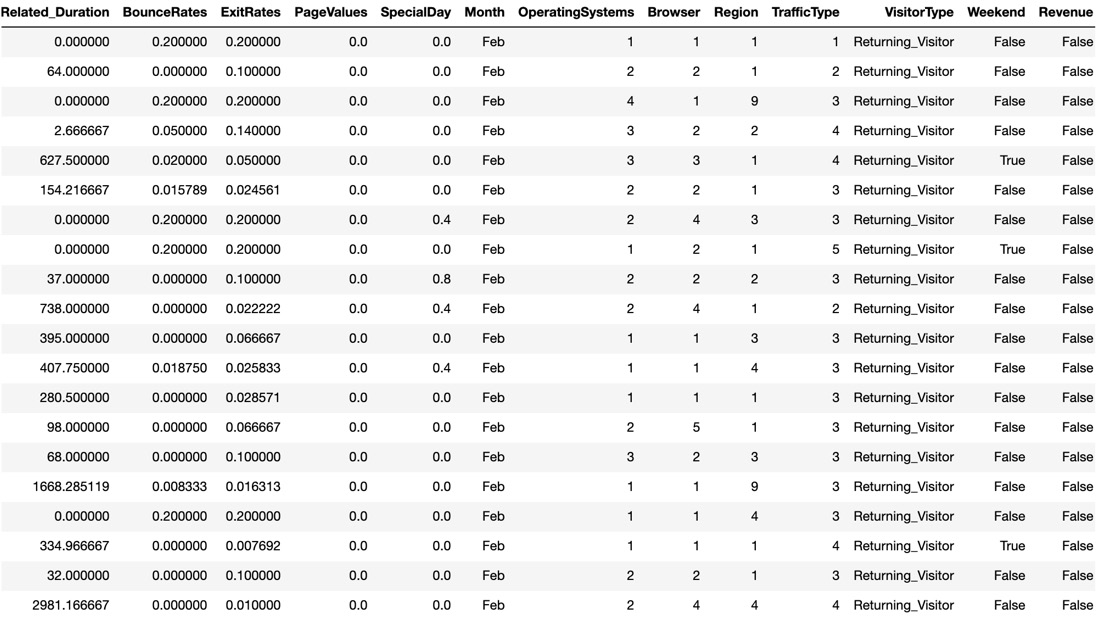
Figure 1.4: An image showing the first 20 instances of the online shoppers purchasing intention dataset
Loading Data
Data can be in different forms and can be available in many places. Datasets for beginners are often given in a flat format, which means that they are two-dimensional, with rows and columns. Other common forms of data may include images, JSON objects, and text documents. Each type of data format has to be loaded in specific ways. For example, numerical data can be loaded into memory using the NumPy library, which is an efficient library for working with matrices in Python.
However, we would not be able to load our marketing data .csv file into memory using the NumPy library because the dataset contains string values. For our dataset, we will use the pandas library because of its ability to easily work with various data types, such as strings, integers, floats, and binary values. In fact, pandas is dependent on NumPy for operations on numerical data types. pandas is also able to read JSON, Excel documents, and databases using SQL queries, which makes the library common among practitioners for loading and manipulating data in Python.
Here is an example of how to load a CSV file using the NumPy library. We use the skiprows argument in case there is a header, which usually contains column names:
import numpy as np
data = np.loadtxt(filename, delimiter=",", skiprows=1)
Here's an example of loading data using the pandas library:
import pandas as pd
data = pd.read_csv(filename, delimiter=",")
Here, we are loading in a .CSV file. The default delimiter is a comma, so passing this as an argument is not necessary but is useful to see. The pandas library can also handle non-numeric datatypes, which makes the library more flexible:
import pandas as pd
data = pd.read_json(filename)
The pandas library will flatten out the JSON and return a DataFrame.
The library can even connect to a database, queries can be fed directly into the function, and the table that's returned will be loaded as a pandas DataFrame:
import pandas as pd
data = pd.read_sql(con, "SELECT * FROM table")
We have to pass a database connection to the function in order for this to work. There is a myriad of ways for this to be achieved, depending on the database flavor.
Other forms of data that are common in deep learning, such as images and text, can also be loaded in and will be discussed later in this course.
You can find all the documentation for pandas here: https://pandas.pydata.org/pandas-docs/stable/. The documentation for NumPy can be found here: https://docs.scipy.org/doc/.
Exercise 1.01: Loading a Dataset from the UCI Machine Learning Repository
Note
For all the exercises and activities in this chapter, you will need to have Python 3.7, Jupyter, and pandas installed on your system. Refer to the Preface for installation instructions. The exercises and activities are performed in Jupyter notebooks. It is recommended to keep a separate notebook for different assignments. You can download all the notebooks from this book's GitHub repository, which can be found here: https://packt.live/2OL5E9t.
In this exercise, we will be loading the online shoppers purchasing intention dataset from the UCI Machine Learning Repository. The goal of this exercise will be to load in the CSV data and identify a target variable to predict and the feature variables to use to model the target variable. Finally, we will separate the feature and target columns and save them to .CSV files so that we can use them in subsequent activities and exercises.
The dataset is related to the online behavior and activity of customers of an online store and indicates whether the user purchased any products from the website. You can find the dataset in the GitHub repository at: https://packt.live/39rdA7S.
Follow these steps to complete this exercise:
- Open a new Jupyter Notebook and load the data into memory using the pandas library with the
read_csvfunction. Import thepandaslibrary and read in thedatafile:import pandas as pd data = pd.read_csv('../data/online_shoppers_intention.csv')Note
The code above assumes that you are using the same folder and file structure as in the GitHub repository. If you get an error that the file cannot be found, then check to make sure your working directory is correctly structured. Alternatively, you can edit the file path in the code so that it points to the correct file location on your system, though you will need to ensure you are consistent with this when saving and loading files in later exercises.
- To verify that we have loaded the data into the memory correctly, we can print the first few rows. Let's print out the top
20values of the variable:data.head(20)
The printed output should look like this:

Figure 1.5: The first 20 rows and first 8 columns of the pandas DataFrame
- We can also print the
shapeof theDataFrame:data.shape
The printed output should look as follows, showing that the DataFrame has
12330rows and18columns:(12330, 18)
We have successfully loaded the data into memory, so now we can manipulate and clean the data so that a model can be trained using this data. Remember that machine learning models require data to be represented as numerical data types in order to be trained. We can see from the first few rows of the dataset that some of the columns are string types, so we will have to convert them into numerical data types later in this chapter.
- We can see that there is a given output variable for the dataset, known as
Revenue, which indicates whether or not the user purchased a product from the website. This seems like an appropriate target to predict, since the design of the website and the choice of the products featured may be based upon the user's behavior and whether they resulted in purchasing a particular product. Createfeatureandtargetdatasets as follows, providing theaxis=1argument:feats = data.drop('Revenue', axis=1) target = data['Revenue']Note
The
axis=1argument tells the function to drop columns rather than rows. - To verify that the shapes of the datasets are as expected, print out the number of
rowsandcolumnsof each:Note
The code snippet shown here uses a backslash (
\) to split the logic across multiple lines. When the code is executed, Python will ignore the backslash, and treat the code on the next line as a direct continuation of the current line.print(f'Features table has {feats.shape[0]} \ rows and {feats.shape[1]} columns') print(f'Target table has {target.shape[0]} rows')This preceding code produces the following output:
Features table has 12330 rows and 17 columns
Target table has 12330 rows
We can see two important things here that we should always verify before continuing: first, the number of rows of the
featureDataFrame andtargetDataFrame are the same. Here, we can see that both have12330rows. Second, the number of columns of the feature DataFrame should be one fewer than the total DataFrame, and the target DataFrame has exactly one column.Regarding the second point, we have to verify that the target is not contained in the feature dataset; otherwise, the model will quickly find that this is the only column needed to minimize the total error, all the way down to zero. The target column doesn't necessarily have to be one column, but for binary classification, as in our case, it will be. Remember that these machine learning models are trying to minimize some cost function in which the
targetvariable will be part of that cost function, usually a difference function between the predicted value andtargetvariable. - Finally, save the DataFrames as CSV files so that we can use them later:
feats.to_csv('../data/OSI_feats.csv', index=False)
target.to_csv('../data/OSI_target.csv', \
              header='Revenue', index=False)
Note
The
header='Revenue'parameter is used to provide a column name. We will do this to reduce confusion later on. Theindex=Falseparameter is used so that the index column is not saved.
In this section, we have successfully demonstrated how to load data into Python using the pandas library. This will form the basis of loading data into memory for most tabular data. Images and large documents, both of which are other common forms of data for machine learning applications, have to be loaded in using other methods, all of which will be discussed later in this book.
Note
To access the source code for this specific section, please refer to https://packt.live/2YZRAyB.
You can also run this example online at https://packt.live/3dVR0pF.