Reader small image

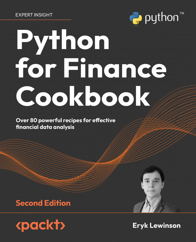
You're reading from  Python for Finance Cookbook - Second Edition

Product typeBook
Published inDec 2022
PublisherPackt
ISBN-139781803243191
Edition2nd Edition
Right arrow
Author (1)
Eryk Lewinson
Eryk Lewinson
author image
Eryk Lewinson

Eryk Lewinson received his master's degree in Quantitative Finance from Erasmus University Rotterdam. In his professional career, he has gained experience in the practical application of data science methods while working in risk management and data science departments of two "big 4" companies, a Dutch neo-broker and most recently the Netherlands' largest online retailer. Outside of work, he has written over a hundred articles about topics related to data science, which have been viewed more than 3 million times. In his free time, he enjoys playing video games, reading books, and traveling with his girlfriend.
Read more about Eryk Lewinson

Right arrow

Backtesting Trading Strategies

In the previous chapters, we gained the knowledge necessary to create trading strategies. On the one hand, we could use technical analysis to identify trading opportunities. On the other, we could use some of the other techniques we have already covered in the book. We could try to use knowledge about factor models or volatility forecasting. Or, we could use portfolio optimization techniques to determine the optimal quantity of assets for our investment. One crucial thing that is still missing is evaluating how such a strategy would have performed if we had implemented it in the past. That is the goal of backtesting, which we explore in this chapter.

Backtesting can be described as a realistic simulation of our trading strategy, which assesses its performance using historical data. The underlying idea is that the backtest performance should be indicative of future performance when the strategy is actually used on the market. Naturally, this will...
Vectorized backtesting with pandas

As we mentioned in the introduction to this chapter, there are two approaches to carrying out backtests. The simpler one is called vectorized backtesting. In this approach, we multiply a signal vector/matrix (containing an indicator of whether we are entering or closing a position) by the vector of returns. By doing so, we calculate the performance over a certain period of time.

Due to its simplicity, this approach cannot deal with many of the issues we described in the introduction, for example:

  • We need to manually align the timestamps to avoid look-ahead bias.
  • There is no explicit position sizing.
  • All performance measurements are calculated manually at the very end of the backtest.
  • Risk-management rules like stop-loss are not easy to incorporate.

That is why we should use vectorized backtesting mostly if we are dealing with simple trading strategies and want to explore their initial potential in a few lines...

Event-driven backtesting with backtrader

The second approach to backtesting is called event-driven backtesting. In this approach, a backtesting engine simulates the time dimension of the trading environment (you can think about it as a for loop going through the time and executing all the actions sequentially). This imposes more structure on the backtest, including the use of historical calendars to define when trades can actually be executed, when prices are available, and so on.

Event-driven backtesting aims to simulate all the actions and constraints encountered when executing a certain strategy while allowing for much more flexibility than the vectorized approach. For example, this approach allows for simulating potential delays in orders’ execution, slippage costs, and so on. In an ideal scenario, a strategy encoded for an event-driven backtest could be easily converted into one working with live trading engines.

Nowadays, there are quite a few event-driven backtesting...

Backtesting a long/short strategy based on the RSI

The relative strength index (RSI) is an indicator that uses the closing prices of an asset to identify oversold/overbought conditions. Most commonly, the RSI is calculated using a 14-day period, and it is measured on a scale from 0 to 100 (it is an oscillator). Traders usually buy an asset when it is oversold (if the RSI is below 30), and sell when it is overbought (if the RSI is above 70). More extreme high/low levels, such as 80-20, are used less frequently and, at the same time, imply stronger momentum.

In this recipe, we build a trading strategy with the following rules:

  • We can go long and short.
  • For calculating the RSI, we use 14 periods (trading days).
  • Enter a long position if the RSI crosses the lower threshold (standard value of 30) upward; exit the position when the RSI becomes larger than the middle level (value of 50).
  • Enter a short position if the RSI crosses the upper threshold (standard...

Backtesting a buy/sell strategy based on Bollinger bands

Bollinger bands are a statistical method, used for deriving information about the prices and volatility of a certain asset over time. To obtain the Bollinger bands, we need to calculate the moving average and standard deviation of the time series (prices), using a specified window (typically 20 days). Then, we set the upper/lower bands at K times (typically 2) the moving standard deviation above/below the moving average.

The interpretation of the bands is quite simple: the bands widen with an increase in volatility and contract with a decrease in volatility.

In this recipe, we build a simple trading strategy that uses Bollinger bands to identify underbought and oversold levels and then trade based on those areas. The rules of the strategy are as follows:

  • Buy when the price crosses the lower Bollinger band upward.
  • Sell (only if stocks are in possession) when the price crosses the upper Bollinger band...

Feedback

We are constantly looking at improving our content, so what could be better than listening to what you as a reader have to say? Your feedback is important to us and we will do our best to incorporate it. Could you take two mins to fill out the feedback form for this book and let us know what your thoughts are about it? Here's the link: https://forms.office.com/r/sYbSyLm2cX.

Thank you in advance.

Asset allocation is the most important decision that any investor needs to face, and there is no one-size-fits-all solution that can work for each and every investor. By asset allocation, we mean spreading the investor's total investment amount over certain assets (be it stocks, options, bonds, or any other financial instruments). When considering the allocation, the investor wants to balance the risk and the potential reward. At the same time, the allocation is dependent on factors such as the individual goals (expected return), risk tolerance (how much risk is the investor...

Evaluating portfolio’s performance on the example of the equally-weighted portfolio

We begin with inspecting the most basic asset allocation strategy: the equally-weighted (1/n) portfolio. The idea is to assign equal weights to all the considered assets, thus diversifying the portfolio. As simple as that might sound, DeMiguel, Garlappi, and Uppal (2007) show that it can be difficult to beat the performance of the 1/n portfolio by using more advanced asset allocation strategies.

The goal of the recipe is to show how to create a 1/n portfolio of the FAANG companies, calculate its returns, and then use the quantstats library to quickly obtain all relevant portfolio evaluation metrics in the form of a tear sheet. Historically, a tear sheet is a concise, usually one-page, document, summarizing important information about public companies.

How to do it...

Execute the following steps to create and evaluate the 1/n portfolio.

  1. Import the libraries:
import yfinance as yf
import numpy...

Finding the Efficient Frontier using Monte Carlo simulations

According to the Modern Portfolio Theory, the Efficient Frontier is a set of optimal portfolios in the risk-return spectrum. This means that the portfolios on the frontier:

  • Offer the highest expected return for a given level of risk,
  • Offer the lowest level of risk for a given level of expected returns.

All portfolios located under the Efficient Frontier curve are considered sub-optimal, so it is always better to choose the ones on the frontier instead.

In this recipe, we show how to find the Efficient Frontier using Monte Carlo simulations. We build thousands of portfolios, using randomly assigned weights, and visualize the results. To do so, we use the returns of the four US tech companies from 202

How to do it...

Execute the following steps to find the Efficient Frontier using Monte Carlo simulations.

  1. Import the libraries:
import yfinance as yf
import numpy as np
import pandas as pd
  1. Set up the parameters:
N_PORTFOLIOS...
lock icon
The rest of the chapter is locked
You have been reading a chapter from
Python for Finance Cookbook - Second Edition
Published in: Dec 2022Publisher: PacktISBN-13: 9781803243191
Register for a free Packt account to unlock a world of extra content!
A free Packt account unlocks extra newsletters, articles, discounted offers, and much more. Start advancing your knowledge today.
undefined
Unlock this book and the full library FREE for 7 days
Get unlimited access to 7000+ expert-authored eBooks and videos courses covering every tech area you can think of
Renews at $15.99/month. Cancel anytime

Author (1)

author image
Eryk Lewinson

Eryk Lewinson received his master's degree in Quantitative Finance from Erasmus University Rotterdam. In his professional career, he has gained experience in the practical application of data science methods while working in risk management and data science departments of two "big 4" companies, a Dutch neo-broker and most recently the Netherlands' largest online retailer. Outside of work, he has written over a hundred articles about topics related to data science, which have been viewed more than 3 million times. In his free time, he enjoys playing video games, reading books, and traveling with his girlfriend.
Read more about Eryk Lewinson