Search icon
Arrow left icon
All Products
Best Sellers
New Releases
Books
Videos
Audiobooks
Learning Hub
Newsletters
Free Learning
Arrow right icon
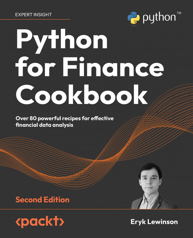
Python for Finance Cookbook - Second Edition

You're reading from  Python for Finance Cookbook - Second Edition

Product type Book
Published in Dec 2022
Publisher Packt
ISBN-13 9781803243191
Pages 740 pages
Edition 2nd Edition
Languages
Author (1):
Eryk Lewinson Eryk Lewinson
Profile icon Eryk Lewinson

Table of Contents (18) Chapters

Preface Acquiring Financial Data Data Preprocessing Visualizing Financial Time Series Exploring Financial Time Series Data Technical Analysis and Building Interactive Dashboards Time Series Analysis and Forecasting Machine Learning-Based Approaches to Time Series Forecasting Multi-Factor Models Modeling Volatility with GARCH Class Models Monte Carlo Simulations in Finance Asset Allocation Backtesting Trading Strategies Applied Machine Learning: Identifying Credit Default Advanced Concepts for Machine Learning Projects Deep Learning in Finance Other Books You May Enjoy
Index

Feedback

We are constantly looking at improving our content, so what could be better than listening to what you as a reader have to say? Your feedback is important to us and we will do our best to incorporate it. Could you take two mins to fill out the feedback form for this book and let us know what your thoughts are about it? Here's the link: https://forms.office.com/r/sYbSyLm2cX.

Thank you in advance.

Time series are omnipresent in both industry and research. We can find examples of time series in commerce, tech, healthcare, energy, finance, and so on. We are mostly interested in the last one, as the time dimension is inherent to trading and many financial/economic indicators. However, pretty much any business generates some sort of time series, for example, its profits collected over time or any other measured KPI. That is why the techniques we cover in the following two chapters can be used for any time series analysis task you might encounter in your line of work.

Time series...

Time series decomposition

One of the goals of time series decomposition is to increase our understanding of the data by breaking down the series into multiple components. It provides insight in terms of modeling complexity and which approaches to follow in order to accurately capture/model each of the components.

An example can shed more light on the possibilities. We can imagine a time series with a clear trend, either increasing or decreasing. On one hand, we could use the decomposition to extract the trend component and remove it from our time series before modeling the remaining series. Then, we can always add it back after the rest of the components are accounted for. On the other hand, we could provide enough data or adequate features for our algorithm to model the trend itself.

The components of time series can be divided into two types: systematic and non-systematic. The systematic ones are characterized by consistency and the fact that they can be described and modeled. By contrast...

Testing for stationarity in time series

One of the most important concepts in time series analysis is stationarity. Plainly speaking a stationary time series is a series whose properties do not depend on the time at which the series is observed. In other words, stationarity implies that the statistical properties of the data-generating process (DGP) of a certain time series do not change over time.

Hence, we should not be able to see any trend or seasonal patterns in a stationary time series, as their existence violates the stationarity assumptions. On the other hand, a white noise process is stationary, as it does not matter when we observe it, it will always look pretty much the same at any point in time.

A time series without trend and seasonality but with cyclic behavior can still be stationary because the cycles are not of a fixed length. So unless we explicitly observe a time series, we cannot be sure where the peaks and troughs of the cycles will be located.

To put it more formally...

Correcting for stationarity in time series

In the previous recipe, we have learned how to investigate if a given time series is stationary. In this one, we investigate how to make a non-stationary time series stationary by using one (or multiple) of the following transformations:

  • deflation - accounting for inflation in monetary series using the Consumer Price Index (CPI)
  • applying the natural logarithm - making the potential exponential trend closer to linear and reducing the variance of the time series
  • differencing - taking the difference between the current observation and a lagged value (observation x time points before it)

For this exercise, we use monthly gold prices from the years 2000 to 2010. We have chosen this sample on purpose, as over that period the price of gold exhibits a consistently increasing trend - the series is definitely not stationary.

How to do it...

Execute the following steps to transform the series from non-stationary to stationary.

  1. Import the libraries...

Modeling time series with exponential smoothing methods

Exponential smoothing methods are one of the two families of classical forecasting models. Their underlying idea is that forecasts are simply weighted averages of past observations. When calculating those averages, more emphasis is put on the recent observations. To achieve that, the weights are decaying exponentially with time. These models are suitable for non-stationary data, that is, data with a trend and/or seasonality. Smoothing methods are popular because they are fast (not a lot of computations are required) and relatively reliable when it comes to forecasts’ accuracy.

Collectively, the exponential smoothing methods can be defined in terms of the ETS framework (Error, Trend, and Season), as they combine the underlying components in the smoothing calculations. As in the case of the seasonal decomposition, those terms can be combined additively, multiplicatively, or simply left out of the model.

Please see Forecasting...

Modeling time series with ARIMA class models

ARIMA models are a class of statistical models that are used for analyzing and forecasting time series data. They aim to do so by describing the autocorrelations in the data. ARIMA stands for Autoregressive Integrated Moving Average and is an extension of a simpler ARMA model. The goal of the additional integration component is to ensure stationarity of the series. That is because, in contrast to the exponential smoothing models, the ARIMA models require the time series to be stationary. Below we briefly go over the models’ building blocks.

AR (autoregressive) model:

  • This kind of model uses the relationship between an observation and its lagged values.
  • In the financial context, the autoregressive model tries to account for the momentum and mean reversion effects.

I (integration):

  • Integration, in this case, refers to differencing the original time series (subtracting the value from the previous period from the current period's...

Finding the best-fitting ARIMA model with auto-ARIMA

As we have seen in the previous recipe, the performance of an ARIMA model varies greatly depending on the chosen hyperparameters (p, d, and q). We can do our best to choose them based on our intuition, the statistical tests, and the ACF/PACF plots. However, this can prove to be quite difficult to do in practice.

That is why in this recipe we introduce auto-ARIMA, an automated approach to finding the best hyperparameters of the ARIMA class models (including variants such as ARIMAX and SARIMA).

Without going much into technical details of the algorithm, it first determines the number of differences using the KPSS test. Then, the algorithm uses a stepwise search to traverse the model space searching for a model that results in a better fit. A popular choice of evaluation metric used for comparing the models is the Akaike Information Criterion (AIC). The metric provides a trade-off between the goodness of fit of the model and its simplicity...

lock icon The rest of the chapter is locked
You have been reading a chapter from
Python for Finance Cookbook - Second Edition
Published in: Dec 2022 Publisher: Packt ISBN-13: 9781803243191
Register for a free Packt account to unlock a world of extra content!
A free Packt account unlocks extra newsletters, articles, discounted offers, and much more. Start advancing your knowledge today.
Unlock this book and the full library FREE for 7 days
Get unlimited access to 7000+ expert-authored eBooks and videos courses covering every tech area you can think of
Renews at $15.99/month. Cancel anytime}