

As mentioned before, pandas is a library for loading, cleaning, and analyzing a variety of different data structures. It is the flexibility of pandas, in addition to the sheer number of built-in features, that makes it such a powerful, popular, and useful Python package. It is also a great package to start with as, obviously, we cannot analyze any data if we do not first load it into the system. As pandas provides so much functionality, one very important skill in using the package is the ability to read and understand the documentation. Even after years of experience programming in Python and using pandas, we still refer to the documentation very frequently. The functionality within the API is so extensive that it is impossible to memorize all of the features and specifics of the implementation.
Note
The pandas documentation can be found at https://pandas.pydata.org/pandas-docs/stable/index.html.
pandas has the ability to read and write a number of different file formats and data structures, including CSV, JSON, and HDF5 files, as well as SQL and Python Pickle formats. The pandas input/output documentation can be found at https://pandas.pydata.org/pandas-docs/stable/user_guide/io.html. We will continue to look into the pandas functionality through loading data via a CSV file. The dataset we will be using for this chapter is the Titanic: Machine Learning from Disaster dataset, available from https://www.kaggle.com/c/Titanic/data or https://github.com/TrainingByPackt/Applied-Supervised-Learning-with-Python, which contains a roll of the guests on board the Titanic as well as their age, survival status, and number of siblings/parents. Before we get started with loading the data into Python, it is critical that we spend some time looking over the information provided for the dataset so that we can have a thorough understanding of what it contains. Download the dataset and place it in the directory you're working in.
Looking at the description for the data, we can see that we have the following fields available:
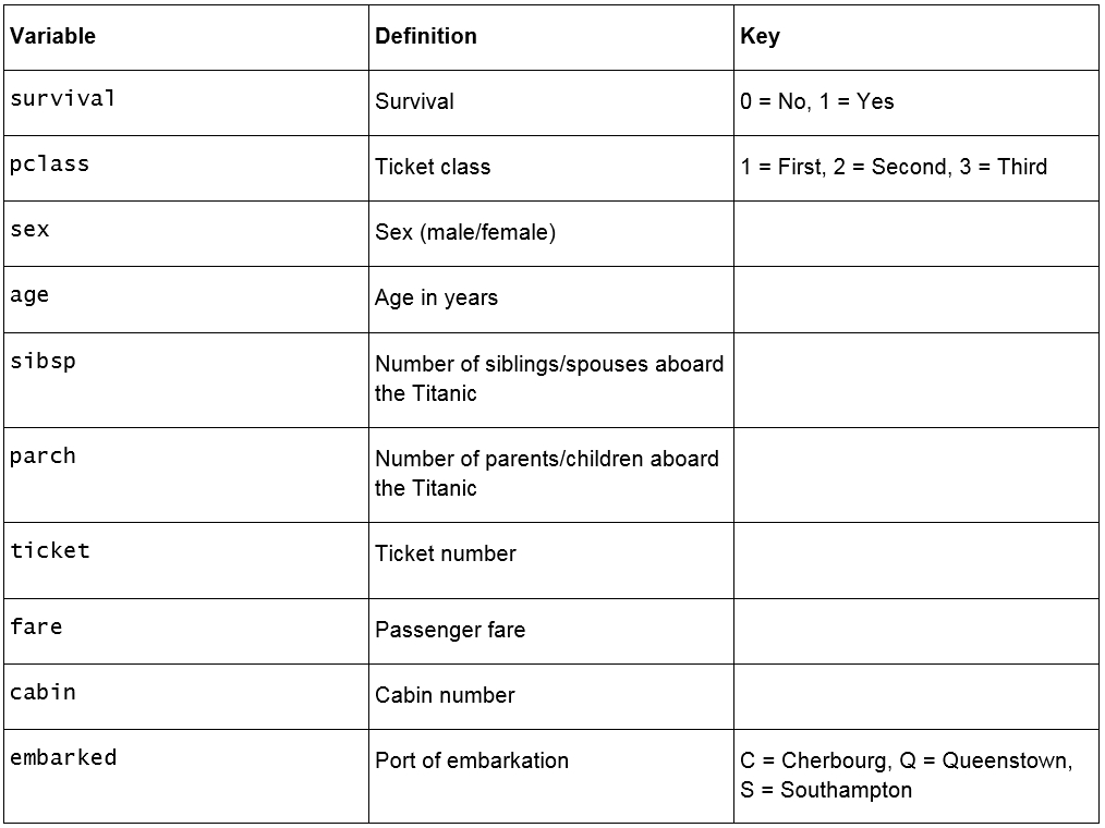
Figure 1.22: Fields in the Titanic dataset
We are also provided with some additional contextual information:
pclass: This is a proxy for socio-economic status, where first class is upper, second class is middle, and third class is lower status.
age: This is a fractional value if less than 1; for example, 0.25 is 3 months. If the age is estimated, it is in the form of xx.5.
sibsp: A sibling is defined as a brother, sister, stepbrother, or stepsister, and a spouse is a husband or wife.
parch: A parent is a mother or father, a child is a daughter, son, stepdaughter, or stepson. Children that traveled only with a nanny did not travel with a parent. Thus, 0 was assigned for this field.
embarked: The point of embarkation is the location where the passenger boarded the ship.
Note that the information provided with the dataset does not give any context as to how the data was collected. The survival, pclass, and embarked fields are known as categorical variables as they are assigned to one of a fixed number of labels or categories to indicate some other information. For example, in embarked, the C label indicates that the passenger boarded the ship at Cherbourg, and the value of 1 in survival indicates they survived the sinking.
In this exercise, we will read our Titanic dataset into Python and perform a few basic summary operations on it:
Import the pandas package using shorthand notation, as shown in the following screenshot:

Figure 1.23: Importing the pandas package
Open the titanic.csv file by clicking on it in the Jupyter notebook home page:

Figure 1.24: Opening the CSV file
The file is a CSV file, which can be thought of as a table, where each line is a row in the table and each comma separates columns in the table. Thankfully, we don't need to work with these tables in raw text form and can load them using pandas:

Figure 1.25: Contents of the CSV file
In an executable Jupyter notebook cell, execute the following code to load the data from the file:
df = pd.read_csv('Titanic.csv')The pandas DataFrame class provides a comprehensive set of attributes and methods that can be executed on its own contents, ranging from sorting, filtering, and grouping methods to descriptive statistics, as well as plotting and conversion.
Read the first five rows of data using the head() method of the DataFrame:
df.head()

Figure 1.26: Reading the first five rows
In this sample, we have a visual representation of the information in the DataFrame. We can see that the data is organized in a tabular, almost spreadsheet-like structure. The different types of data are organized by columns, while each sample is organized by rows. Each row is assigned to an index value and is shown as the numbers 0 to 4 in bold on the left-hand side of the DataFrame. Each column is assigned to a label or name, as shown in bold at the top of the DataFrame.
The idea of a DataFrame as a kind of spreadsheet is a reasonable analogy; as we will see in this chapter, we can sort, filter, and perform computations on the data just as you would in a spreadsheet program. While not covered in this chapter, it is interesting to note that DataFrames also contain pivot table functionality, just like a spreadsheet (https://pandas.pydata.org/pandas-docs/stable/reference/api/pandas.pivot_table.html).
Now that we have loaded some data, let's use the selection and indexing methods of the DataFrame to access some data of interest:
Select individual columns in a similar way to a regular dictionary, by using the labels of the columns, as shown here:
df['Age']

Figure 1.27: Selecting the Age column
If there are no spaces in the column name, we can also use the dot operator. If there are spaces in the column names, we will need to use the bracket notation:
df.Age

Figure 1.28: Using the dot operator to select the Age column
Select multiple columns at once using bracket notation, as shown here:
df[['Name', 'Parch', 'Sex']]

Figure 1.29: Selecting multiple columns
Select the first row using iloc:
df.iloc[0]

Figure 1.30: Selecting the first row
Select the first three rows using iloc:
df.iloc[[0,1,2]]

Figure 1.31: Selecting the first three rows
We can also get a list of all of the available columns. Do this as shown here:
columns = df.columns # Extract the list of columns
print(columns)

Figure 1.32: Getting all the columns
Use this list of columns and the standard Python slicing syntax to get columns 2, 3, and 4, and their corresponding values:
df[columns[1:4]] # Columns 2, 3, 4

Figure 1.33: Getting the second, third, and fourth columns
Use the len operator to get the number of rows in the DataFrame:
len(df)

Figure 1.34: Getting the number of rows
What if we wanted the value for the Fare column at row 2? There are a few different ways to do so. First, we'll try the row-centric methods. Do this as follows:
df.iloc[2]['Fare'] # Row centric

Figure 1.35: Getting a particular value using the normal row-centric method
Try using the dot operator for the column. Do this as follows:
df.iloc[2].Fare # Row centric

Figure 1.36: Getting a particular value using the row-centric dot operator
Try using the column-centric method. Do this as follows:
df['Fare'][2] # Column centric

Figure 1.37: Getting a particular value using the normal column-centric method
Try the column-centric method with the dot operator. Do this as follows:
df.Fare[2] # Column centric

Figure 1.38: Getting a particular value using the column-centric dot operator
With the basics of indexing and selection under our belt, we can turn our attention to more advanced indexing and selection. In this exercise, we will look at a few important methods for performing advanced indexing and selecting data:
Create a list of the passengers' names and ages for those passengers under the age of 21, as shown here:
child_passengers = df[df.Age  < 21][['Name', 'Age']]
child_passengers.head()

Figure 1.39: List of the passengers' names and ages for those passengers under the age of 21
Count how many child passengers there were, as shown here:
print(len(child_passengers))

Figure 1.40: Count of child passengers
Count how many passengers were between the ages of 21 and 30. Do not use Python's and logical operator for this step, but rather the ampersand symbol (&). Do this as follows:
young_adult_passengers = df.loc[
    (df.Age > 21) & (df.Age < 30)
]
len(young_adult_passengers)
Figure 1.41: Count of passengers between the ages of 21 and 30
Count the passengers that were either first- or third-class ticket holders. Again, we will not use the Python logical or operator but rather the pipe symbol (|). Do this as follows:
df.loc[
    (df.Pclass == 3) | (df.Pclass ==1)
]
Figure 1.42: Count of passengers that were either first- or third-class ticket holders
Count the passengers who were not holders of either first- or third-class tickets. Do not simply select the second class ticket holders, but rather use the ~ symbol for the not logical operator. Do this as follows:
df.loc[
    ~((df.Pclass == 3) | (df.Pclass ==1))
]
Figure 1.43: Count of passengers who were not holders of either first- or third-class tickets
We no longer need the Unnamed: 0 column, so delete it using the del operator:
del df['Unnamed: 0']
df.head()

Figure 1.44: The del operator
Now that we are confident with some pandas basics, as well as some more advanced indexing and selecting tools, let's look at some other DataFrame methods. For a complete list of all methods available in a DataFrame, we can refer to the class documentation.
Note
The pandas documentation is available at https://pandas.pydata.org/pandas-docs/stable/reference/frame.html.
You should now know how many methods are available within a DataFrame. There are far too many to cover in detail in this chapter, so we will select a few that will give you a great start in supervised machine learning.
We have already seen the use of one method, head(), which provides the first five lines of the DataFrame. We can select more or less lines if we wish, by providing the number of lines as an argument, as shown here:
df.head(n=20) # 20 lines
df.head(n=32) # 32 lines
Another useful method is describe, which is a super-quick way of getting the descriptive statistics of the data within a DataFrame. We can see next that the sample size (count), mean, minimum, maximum, standard deviation, and 25th, 50th, and 75th percentiles are returned for all columns of numerical data in the DataFrame (note that text columns have been omitted):
df.describe()
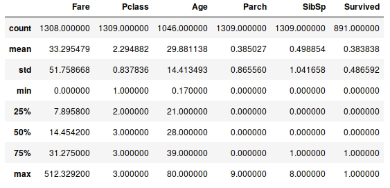
Figure 1.45: The describe method
Note that only columns of numerical data have been included within the summary. This simple command provides us with a lot of useful information; looking at the values for count (which counts the number of valid samples), we can see that there are 1,046 valid samples in the Age category, but 1,308 in Fare, and only 891 in Survived. We can see that the youngest person was 0.17 years, the average age is 29.898, and the eldest 80. The minimum fare was £0, with £33.30 the average and £512.33 the most expensive. If we look at the Survived column, we have 891 valid samples, with a mean of 0.38, which means about 38% survived.
We can also get these values separately for each of the columns by calling the respective methods of the DataFrame, as shown here:
df.count()
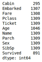
Figure 1.46: The count method
But we have some columns that contain text data, such as Embarked, Ticket, Name, and Sex. So, what about these? How can we get some descriptive information for these columns? We can still use describe; we just need to pass it some more information. By default, describe will only include numerical columns and will compute the 25th, 50th, and 75th percentiles. But we can configure this to include text-based columns by passing the include = 'all' argument, as shown here:
df.describe(include='all')
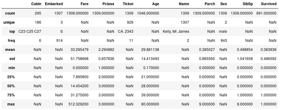
Figure 1.47: The describe method with text-based columns
That's better—now we have much more information. Looking at the Cabin column, we can see that there are 295 entries, with 186 unique values. The most common values are C32, C25, and C27, and they occur 6 times (from the freq value). Similarly, if we look at the Embarked column, we see that there are 1,307 entries, 3 unique values, and that the most commonly occurring value is S with 914 entries.
Notice the occurrence of NaN values in our describe output table. NaN, or Not a Number, values are very important within DataFrames, as they represent missing or not available data. The ability of the pandas library to read from data sources that contain missing or incomplete information is both a blessing and a curse. Many other libraries would simply fail to import or read the data file in the event of missing information, while the fact that it can be read also means that the missing data must be handled appropriately.
When looking at the output of the describe method, you should notice that the Jupyter notebook renders it in the same way as the original DataFrame that we read in using read_csv. There is a very good reason for this, as the results returned by the describe method are themselves a pandas DataFrame and thus possess the same methods and characteristics as the data read in from the CSV file. This can be easily verified using Python's built-in type function:
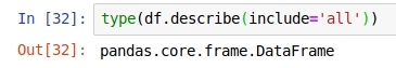
Figure 1.48: Checking the type
Now that we have a summary of the dataset, let's dive in with a little more detail to get a better understanding of the available data.
Note
A comprehensive understanding of the available data is critical in any supervised learning problem. The source and type of the data, the means by which it is collected, and any errors potentially resulting from the collection process all have an effect on the performance of the final model.
Hopefully, by now, you are comfortable with using pandas to provide a high-level overview of the data. We will now spend some time looking into the data in greater detail.
We have already seen how we can index or select rows or columns from a DataFrame and use advanced indexing techniques to filter the available data based on specific criteria. Another handy method that allows for such selection is the groupby method, which provides a quick method for selecting groups of data at a time and provides additional functionality through the DataFrameGroupBy object:
Use the groupby method to group the data by the Embarked column. How many different values for Embarked are there? Let's see:
embarked_grouped = df.groupby('Embarked')

print(f'There are {len(embarked_grouped)} Embarked groups')
Figure 1.49: Grouping the data by the Embarked column
What does the groupby method actually do? Let's check. Display the output of embarked_grouped.groups:
embarked_grouped.groups

Figure 1.50: Output of embarked_grouped.groups
We can see here that the three groups are C, Q, and S, and that embarked_grouped.groups is actually a dictionary where the keys are the groups. The values are the rows or indexes of the entries that belong to that group.
Use the iloc method to inspect row 1 and confirm that it belongs to embarked group C:
df.iloc[1]

Figure 1.51: Inspecting row 1
As the groups are a dictionary, we can iterate through them and execute computations on the individual groups. Compute the mean age for each group, as shown here:
for name, group in embarked_grouped:
    print(name, group.Age.mean())
Figure 1.52: Computing the mean age for each group using iteration
Another option is to use the aggregate method, or agg for short, and provide it the function to apply across the columns. Use the agg method to determine the mean of each group:
embarked_grouped.agg(np.mean)

Figure 1.53: Using the agg method
So, how exactly does agg work and what type of functions can we pass it? Before we can answer these questions, we need to first consider the data type of each column in the DataFrame, as each column is passed through this function to produce the result we see here. Each DataFrame is comprised of a collection of columns of pandas series data, which in many ways operates just like a list. As such, any function that can take a list or a similar iterable and compute a single value as a result can be used with agg.
As an example, define a simple function that returns the first value in the column, then pass that function through to agg:
def first_val(x):

    return x.values[0]

embarked_grouped.agg(first_val)
Figure 1.54: Using the agg method with a function
One common and useful way of implementing agg is through the use of Lambda functions.
Lambda or anonymous functions (also known as inline functions in other languages) are small, single-expression functions that can be declared and used without the need for a formal function definition via use of the def keyword. Lambda functions are essentially provided for convenience and aren't intended to be used for extensive periods. The standard syntax for a Lambda function is as follows (always starting with the lambda keyword):
lambda <input values>: <computation for values to be returned>
In this exercise, we will create a Lambda function that returns the first value in a column and use it with agg:
Write the first_val function as a Lambda function, passed to agg:
embarked_grouped.agg(lambda x: x.values[0])

Figure 1.55: Using the agg method with a Lambda function
Obviously, we get the same result, but notice how much more convenient the Lambda function was to use, especially given the fact that it is only intended to be used briefly.
We can also pass multiple functions to agg via a list to apply the functions across the dataset. Pass the Lambda function as well as the NumPy mean and standard deviation functions, like this:
embarked_grouped.agg([lambda x: x.values[0], np.mean, np.std])

Figure 1.56: Using the agg method with multiple Lambda functions
What if we wanted to apply different functions to different columns in the DataFrame? Apply numpy.sum to the Fare column and the Lambda function to the Age column by passing agg a dictionary where the keys are the columns to apply the function to and the values are the functions themselves:
embarked_grouped.agg({
    'Fare': np.sum,
    'Age': lambda x: x.values[0]
})
Figure 1.57: Using the agg method with a dictionary of different columns
Finally, you can also execute the groupby method using more than one column. Provide the method with a list of the columns (Sex and Embarked) to groupby, like this:
age_embarked_grouped = df.groupby(['Sex', 'Embarked'])
age_embarked_grouped.groups

Figure 1.58: Using the groupby method with more than one column
Similar to when the groupings were computed by just the Embarked column, we can see here that a dictionary is returned where the keys are the combination of the Sex and Embarked columns returned as a tuple. The first key-value pair in the dictionary is a tuple, ('Male', 'S'), and the values correspond to the indices of rows with that specific combination. There will be a key-value pair for each combination of unique values in the Sex and Embarked columns.