

1.4 A probability primer for Bayesian practitioners
In this section, we are going to discuss a few general and important concepts that are key for better understanding Bayesian methods. Additional probability-related concepts will be introduced or elaborated on in future chapters, as we need them. For a detailed study of probability theory, however, I highly recommend the book Introduction to Probability by Blitzstein [2019]. Those already familiar with the basic elements of probability theory can skip this section or skim it.
1.4.1 Sample space and events
Let’s say we are surveying to see how people feel about the weather in their area. We asked three individuals whether they enjoy sunny weather, with possible responses being “yes” or “no.” The sample space of all possible outcomes can be denoted by S and consists of eight possible combinations:
S = {(yes, yes, yes), (yes, yes, no), (yes, no, yes), (no, yes, yes), (yes, no, no), (no, yes, no), (no, no, yes), (no, no, no)}
Here, each element of the sample space represents the responses of the three individuals in the order they were asked. For example, (yes, no, yes) means the first and third people answered “yes” while the second person answered “no.”
We can define events as subsets of the sample space. For example, event A is when all three individuals answered “yes”:
A = {(yes, yes, yes)}
Similarly, we can define event B as when at least one person answered “no,” and then we will have:
B = {(yes, yes, no), (yes, no, yes), (no, yes, yes), (yes, no, no), (no, yes, no), (no, no, yes), (no, no, no)}
We can use probabilities as a measure of how likely these events are. Assuming all events are equally likely, the probability of event A, which is the event that all three individuals answered “yes,” is:
In this case, there is only one outcome in A, and there are eight outcomes in S. Therefore, the probability of A is:
Similarly, we can calculate the probability of event B, which is the event that at least one person answered “no.” Since there are seven outcomes in B and eight outcomes in S, the probability of B is:
Considering all events equally likely is just a particular case that makes calculating probabilities easier. This is something called the naive definition of probability since it is restrictive and relies on strong assumptions. However, it is still useful if we are cautious when using it. For instance, it is not true that all yes-no questions have a 50-50 chance. Another example. What is the probability of seeing a purple horse? The right answer can vary a lot depending on whether we’re talking about the natural color of a real horse, a horse from a cartoon, a horse dressed in a parade, etc. Anyway, no matter if the events are equally likely or not, the probability of the entire sample space is always equal to 1. We can see that this is true by computing:
1 is the highest value a probability can take. Saying that P(S) = 1 is saying that S is not only very likely, it is certain. If everything that can happen is defined by S, then S will happen.
If an event is impossible, then its probability is 0. Let’s define the event C as the event of three persons saying “banana”:
C = {(banana, banana, banana)}
As C is not part of S, by definition, it cannot happen. Think of this as the questionnaire from our survey only having two boxes, yes and no. By design, our survey is restricting all other possible options.
We can take advantage of the fact that Python includes sets and define a Python function to compute probabilities following their naive definition:
Code 1.1
def P(S, A):if set(A).issubset(set(S)):return len(A)/len(S)else:return 0
I left for the reader the joy of playing with this function.
One useful way to conceptualize probabilities is as conserved quantities distributed throughout the sample space. This means that if the probability of one event increases, the probability of some other event or events must decrease so that the total probability remains equal to 1. This can be illustrated with a simple example.
Suppose we ask one person whether it will rain tomorrow, with possible responses of “yes” and “no.” The sample space for possible responses is given by S = {yes, no}. An event that will rain tomorrow is represented by A = {yes}. If P(A), is 0.5, then the probability of the complement of event A, denoted by P , must also be 0.5. If for some reason P(A) increases to 0.8, then P
 must decrease to 0.2. This property holds for disjoint events, which are events that cannot occur simultaneously. For instance, it cannot rain and not rain at the same time tomorrow. You may object that it can rain during the morning and not rain during the afternoon. That is true, but that’s a different sample space!
So far, we have avoided directly defining probabilities, and instead, we have just shown some of their properties and ways to compute them. A general definition of probability that works for non-equally likely events is as follows. Given a sample space S, and the event A, which is a subset of S, a probability is a function P, which takes A as input and returns a real number between 0 and 1, as output. The function P has some restrictions, defined by the following 3 axioms. Keep in mind that an axiom is a statement that is taken to be true and that we use as the starting point in our reasoning:
The probability of an event is a non-negative real number
P(S) = 1
If A1,A2,… are disjoint events, meaning they cannot occur simultaneously then P(A1,A2,…) = P(A1) + P(A2) + …
If this were a book on probability theory, we would likely dedicate a few pages to demonstrating the consequences of these axioms and provide exercises for manipulating probabilities. That would help us to become proficient in manipulating probabilities. However, our main focus is not on those topics. My motivation to present these axioms is just to show that probabilities are well-defined mathematical concepts with rules that govern their operations. They are a particular type of function, and there is no mystery surrounding them.
1.4.2 Random variables
A random variable is a function that maps the sample space into the real numbers ℝ (see Figure 1.1). Let’s assume the events of interest are the number of a die, the mapping is very simple, we associate ![]() with the number 1,
with the number 1, ![]() with 2, etc. Another simple example is the answer to the question, will it rain tomorrow? We can map “yes” to 1 and “no” to 0. It is common, but not always the case, to use a capital letter for random variables like X and a lowercase letter for their outcomes x. For example, if X represents a single roll of a die, then x represents some specific integer {1,2,3,4,5,6}. Thus, we can write P(X = 3) to indicate the probability of getting the value 3, when rolling a die. We can also leave x unspecified, for instance, we can write P(X = x) to indicate the probability of getting some value x, or P(X ≤ x), to indicate the probability of getting a value less than or equal to x.
with 2, etc. Another simple example is the answer to the question, will it rain tomorrow? We can map “yes” to 1 and “no” to 0. It is common, but not always the case, to use a capital letter for random variables like X and a lowercase letter for their outcomes x. For example, if X represents a single roll of a die, then x represents some specific integer {1,2,3,4,5,6}. Thus, we can write P(X = 3) to indicate the probability of getting the value 3, when rolling a die. We can also leave x unspecified, for instance, we can write P(X = x) to indicate the probability of getting some value x, or P(X ≤ x), to indicate the probability of getting a value less than or equal to x.
Being able to map symbols like ![]() or strings like “yes” to numbers makes analysis simpler as we already know how to do math with numbers. Random variables are also useful because we can operate with them without directly thinking in terms of the sample space. This feature becomes more and more relevant as the sample space becomes more complex. For example, when simulating molecular systems, we need to specify the position and velocity of each atom; for complex molecules like proteins this means that we will need to track thousands, millions, or even larger numbers. Instead, we can use random variables to summarize certain properties of the system, such as the total energy or the relative angles between certain atoms of the system.
or strings like “yes” to numbers makes analysis simpler as we already know how to do math with numbers. Random variables are also useful because we can operate with them without directly thinking in terms of the sample space. This feature becomes more and more relevant as the sample space becomes more complex. For example, when simulating molecular systems, we need to specify the position and velocity of each atom; for complex molecules like proteins this means that we will need to track thousands, millions, or even larger numbers. Instead, we can use random variables to summarize certain properties of the system, such as the total energy or the relative angles between certain atoms of the system.
If you are still confused, that’s fine. The concept of a random variable may sound too abstract at the beginning, but we will see plenty of examples throughout the book that will help you cement these ideas. Before moving on, let me try one analogy that I hope you find useful. Random variables are useful in a similar way to how Python functions are useful. We often encapsulate code within functions, so we can store, reuse, and hide complex manipulations of data into a single call. Even more, once we have a few functions, we can sometimes combine them in many ways, like adding the output of two functions or using the output of one function as the input of the other. We can do all this without functions, but abstracting away the inner workings not only makes the code cleaner, it also helps with understanding and fostering new ideas. Random variables play a similar role in statistics.
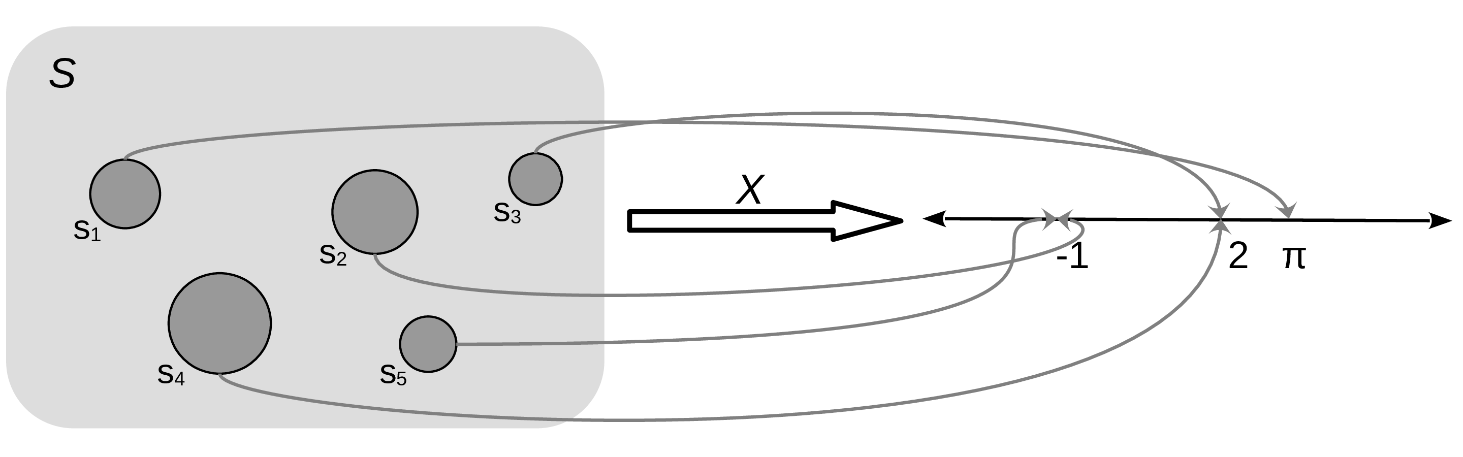
Figure 1.1: A random variable X defined on a sample space with 5 elements {S1, S5}, and possible values -1, 2, and π
The mapping between the sample space and ℝ is deterministic. There is no randomness involved. So why do we call it a random variable? Because we can ask the variable for values, and every time we ask, we will get a different number. The randomness comes from the probability associated with the events. In Figure 1.1, we have represented P as the size of the circles.
The two most common types of random variables are discrete and continuous ones. Without going into a proper definition, we are going to say that discrete variables take only discrete values and we usually use integers to represent them, like 1, 5, 42. And continuous variables take real values, so we use floats to work with them, like 3.1415, 1.01, 23.4214, and so on. When we use one or the other is problem-dependent. If we ask people about their favorite color, we will get answers like “red,” “blue,” and “green.” This is an example of a discrete random variable. The answers are categories – there are no intermediate values between “red” and “green.” But if we are studying the properties of light absorption, then discrete values like “red” and “green” may not be adequate and instead working with wavelength could be more appropriate. In that case, we will expect to get values like 650 nm and 510 nm and any number in between, including 579.1.
1.4.3 Discrete random variables and their distributions
Instead of calculating the probability that all three individuals answered “yes,” or the probability of getting a 3 when rolling a die, we may be more interested in finding out the list of probabilities for all possible answers or all possible numbers from a die. Once this list is computed, we can inspect it visually or use it to compute other quantities like the probability of getting at least one “no,” the probability of getting an odd number, or the probability of getting a number equal to or larger than 5. The formal name of this list is probability distribution.
We can get the empirical probability distribution of a die, by rolling it a few times and tabulating how many times we got each number. To turn each value into a probability and the entire list into a valid probability distribution, we need to normalize the counts. We can do this by dividing the value we got for each number by the number of times we roll the die.
Empirical distributions are very useful, and we are going to extensively use them. But instead of rolling dice by hand, we are going to use advanced computational methods to do the hard work for us; this will not only save us time and boredom but it will allow us to get samples from really complicated distributions effortlessly. But we are getting ahead of ourselves. Our priority is to concentrate on theoretical distributions, which are central in statistics because, among other reasons, they allow the construction of probabilistic models.
As we saw, there is nothing random or mysterious about random variables; they are just a type of mathematical function. The same goes for theoretical probability distributions. I like to compare probability distributions with circles. Because we are all familiar with circles even before we get into school, we are not afraid of them and they don’t look mysterious to us. We can define a circle as the geometric space of points on a plane that is equidistant from another point called the center. We can go further and provide a mathematical expression for this definition. If we assume the location of the center is irrelevant, then the circle of radius r can simply be described as the set of all points (x,y) such that:
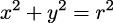
From this expression, we can see that given the parameter r, the circle is completely defined. This is all we need to plot it and all we need to compute properties such as the perimeter, which is 2πr.
Now notice that all circles look very similar to each other and that any two circles with the same value of r are essentially the same objects. Thus we can think of the family of circles, where each member is set apart from the rest precisely by the value of r.
So far, so good, but why are we talking about circles? Because all this can be directly applied to probability distributions. Both circles and probability distributions have mathematical expressions that define them, and these expressions have parameters that we can change to define all members of a family of probability distributions. Figure 1.2 shows four members of one probability distribution known as BetaBinomial. In Figure 1.2, the height of the bars represents the probability of each x value. The values of x below 1 or above 6 have a probability of 0 as they are out of the support of the distribution.
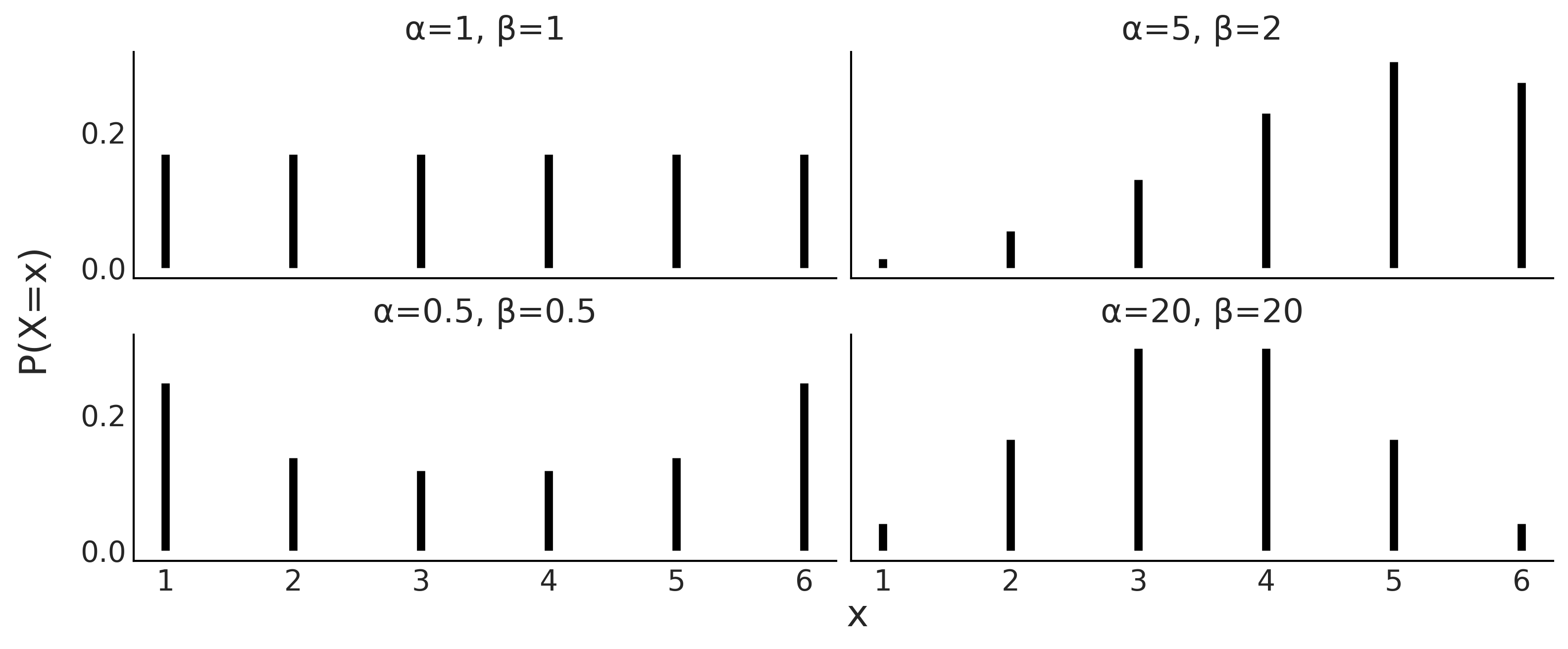
Figure 1.2: Four members of the BetaBinomial distribution with parameters α and β
This is the mathematical expression for the BetaBinomial distribution:
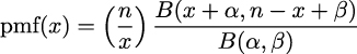
pmf stands for probability mass function. For discrete random variables, the pmf is the function that returns probabilities. In mathematical notation, if we have a random variable X, then pmf(x) = P(X = x).
Understanding or remembering the pmf of the BetaBinomial has zero importance for us. I’m just showing it here so you can see that this is just another function; you put in one number and you get out another number. Nothing weird, at least not in principle. I must concede that to fully understand the details of the BetaBinomial distribution, we need to know what  is, known as the binomial coefficient, and what B is, the Beta function. But that’s not fundamentally different from showing x2 + y2 = r2.
Mathematical expressions can be super useful, as they are concise and we can use them to derive properties from them. But sometimes that can be too much work, even if we are good at math. Visualization can be a good alternative (or complement) to help us understand probability distributions. I cannot fully show this on paper, but if you run the following, you will get an interactive plot that will update every time you move the sliders for the parameters alpha, beta, and n:
Code 1.2
pz.BetaBinomial(alpha=10, beta=10, n=6).plot_interactive()Figure 1.3 shows a static version of this interactive plot. The black dots represent the probabilities for each value of the random variable, while the dotted black line is just a visual aid.
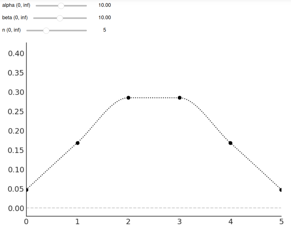
Figure 1.3: The output of pz.BetaBinomial(alpha=10, beta=10, n=6).plot_interactive()
On the x-axis, we have the support of the BetaBinomial distribution, i.e., the values it can take, x ∈{0,1,2,3,4,5}. On the y-axis, the probabilities associated with each of those values. The full list is shown in Table 1.1.
| x value | probability |
| 0 | 0.047 |
| 1 | 0.168 |
| 2 | 0.285 |
| 3 | 0.285 |
| 4 | 0.168 |
| 5 | 0.047 |
Table 1.1: Probabilities for pz.BetaBinomial(alpha=10, beta=10, n=6)
Notice that for a BetaBinomial(alpha=10, beta=10, n=6) distribution, the probability of values not in {0,1,2,3,4,5}, including values such as −1,0.5,π,42, is 0.
We previously mentioned that we can ask a random variable for values and every time we ask, we will get a different number. We can simulate this with PreliZ [Icazatti et al., 2023], a Python library for prior elicitation. Take the following code snippet for instance:
Code 1.3
pz.BetaBinomial(alpha=10, beta=10, n=6).rvs()This will give us an integer between 0 and 5. Which one? We don’t know! But let’s run the following code:
Code 1.4
plt.hist(pz.BetaBinomial(alpha=2, beta=5, n=5).rvs(1000))pz.BetaBinomial(alpha=2, beta=5, n=5).plot_pdf();
We will get something similar to Figure 1.4. Even when we cannot predict the next value from a random variable, we can predict the probability of getting any particular value and by the same token, if we get many values, we can predict their overall distribution.
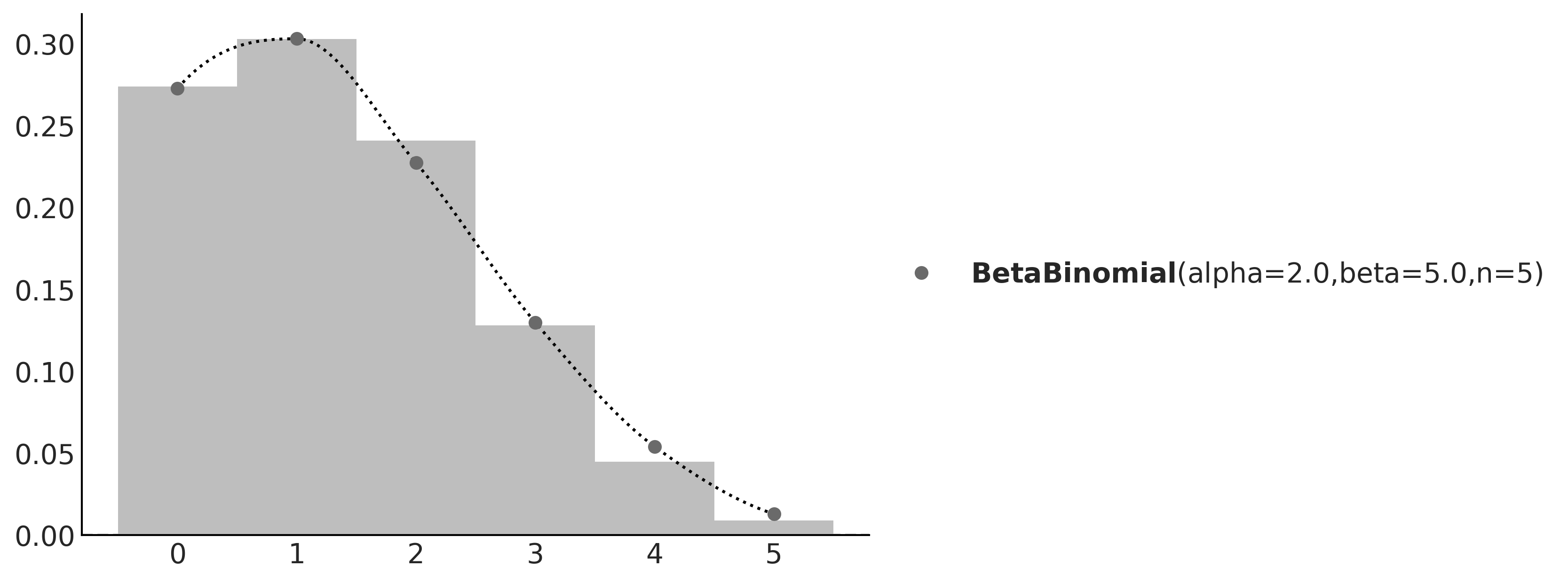
Figure 1.4: The gray dots represent the pmf of the BetaBinomial sample. In light gray, a histogram of 1,000 draws from that distribution
In this book, we will sometimes know the parameters of a given distribution and we will want to get random samples from it. Other times, we are going to be in the opposite scenario: we will have a set of samples and we will want to estimate the parameters of a distribution. Playing back and forth between these two scenarios will become second nature as we move forward through the pages.
1.4.4 Continuous random variables and their distributions
Probably the most widely known continuous probability distribution is the Normal distribution, also known as the Gaussian distribution. Its probability density function is:
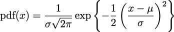
Again, we only show this expression to remove the mystery veil. No need to pay too much attention to its details, other than to the fact that this distribution has two parameters μ, which controls the location of the peak of the curve, and σ, which controls the spread of the curve. Figure 1.5 shows 3 examples from the Gaussian family. If you want to learn more about this distribution, I recommend you watch this video: https://www.youtube.com/watch?v=cy8r7WSuT1I.
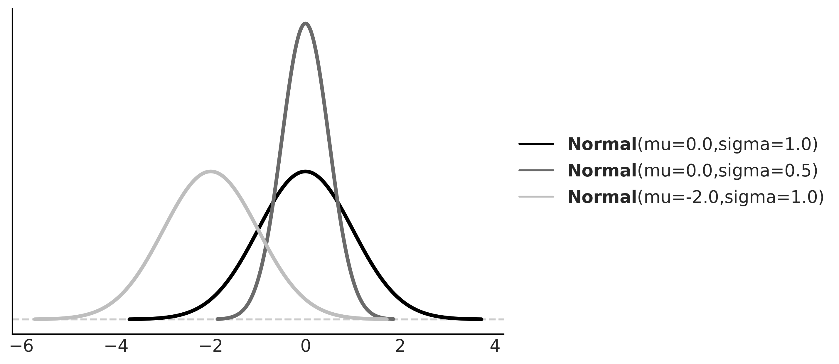
Figure 1.5: Three members of the Gaussian family
If you have been paying attention, you may have noticed that we said probability density function (pdf) instead of probability mass function (pmf). This was no typo – they are actually two different objects. Let’s take one step back and think about this; the output of a discrete probability distribution is a probability. The height of the bars in Figure 1.2 or the height of the dots in Figure 1.3 are probabilities. Each bar or dot will never be higher than 1 and if you sum all the bars or dots, you will always get 1. Let’s do the same but with the curve in Figure 1.5. The first thing to notice is that we don’t have bars or dots; we have a continuous, smooth curve. So maybe we can think that the curve is made up of super thin bars, so thin that we assign one bar for every real value in the support of the distributions, we measure the height of each bar, and we perform an infinite sum. This is a sensible thing to do, right?
Well yes, but it is not immediately obvious what are we going to get from this. Will this sum give us exactly 1? Or are we going to get a large number instead? Is the sum finite? Or does the result depend on the parameters of the distribution?
A proper answer to these questions requires measure theory, and this is a very informal introduction to probability, so we are not going into that rabbit hole. But the answer essentially is that for a continuous random variable, we can only assign a probability of 0 to every individual value it may take; instead, we can assign densities to them and then we can calculate probabilities for a range of values. Thus, for a Gaussian, the probability of getting exactly the number -2, i.e. the number -2 followed by an infinite number of zeros after the decimal point, is 0. But the probability of getting a number between -2 and 0 is some number larger than 0 and smaller than 1. To find out the exact answer, we need to compute the following:
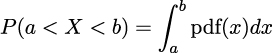
And to compute that, we need to replace the symbols for a concrete quantity. If we replace the pdf by Normal(0,1), and a = −2, b = 0, we will get that P(−2 < X < 0) ≈ 0.477, which is the shaded area in Figure 1.6.
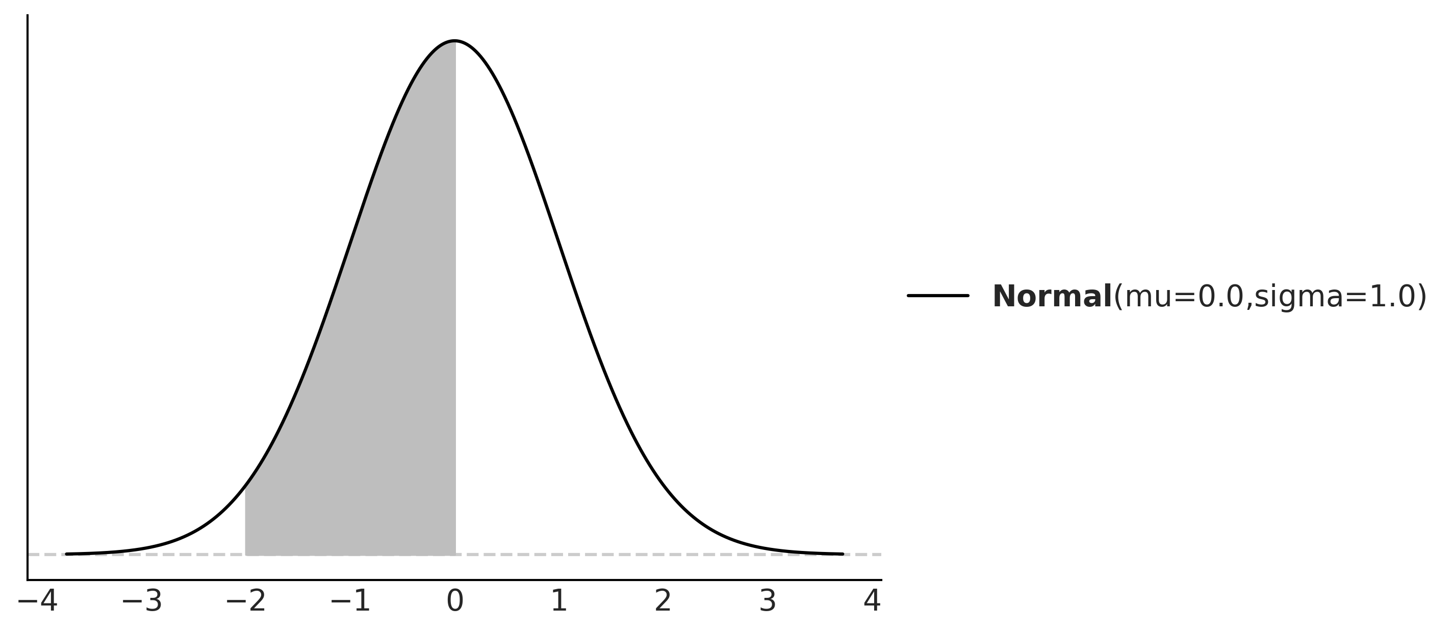
Figure 1.6: The black line represents the pdf of a Gaussian with parameters mu=0 and sigma=1, the gray area is the probability of a value being larger than -2 and smaller than 0
You may remember that we can approximate an integral by summing areas of rectangles and the approximation becomes more and more accurate as we reduce the length of the base of the rectangles (see the Wikipedia entry for Riemann integral). Based on this idea and using PreliZ, we can estimate P(−2 < X < 0) as:
Code 1.5
dist = pz.Normal(0, 1)a = -2b = 0num = 10x_s = np.linspace(a, b, num)base = (b-a)/numnp.sum(dist.pdf(x_s) * base)
If we increase the value of num, we will get a better approximation.
1.4.5 Cumulative distribution function
We have seen the pmf and the pdf, but these are not the only ways to characterize distributions. An alternative is the cumulative distribution function (cdf). The cdf of a random variable X is the function FX given by FX(x) = P(X ≤ x). In words, the cdf is the answer to the question: what is the probability of getting a number lower than or equal to x? On the first column of Figure 1.7, we can see the pmf and cdf of a BetaBinomial, and in the second column, the pdf and cdf of a Gaussian. Notice how the cdf jumps for the discrete variable but it is smooth for the continuous variable. The height of each jump represents a probability – just compare them with the height of the dots. We can use the plot of the cdf of a continuous variable as visual proof that probabilities are zero for any value of the continuous variable. Just notice how there are no jumps for continuous variables, which is equivalent to saying that the height of the jumps is exactly zero.
Figure 1.7: The pmf of the BetaBinomial distribution with its corresponding cdf and the pdf of the Normal distribution with its corresponding cdf
Just by looking at a cdf, it is easier to find what is the probability of getting a number smaller than, let’s say, 1. We just need to go to the value 1 on the x-axis, move up until we cross the black line, and then check the value of the y-axis. For instance, in Figure 1.7 and for the Normal distribution, we can see that the value lies between 0.75 and 1. Let’s say it is ≈ 0.85. This is way harder to do with the pdf because we would need to compare the entire area below 1 to the total area to get the answer. Humans are worse at judging areas than judging heights or lengths.
1.4.6 Conditional probability
Given two events A and B with P(B) > 0, the probability of A given B, which we write as P(A|B) is defined as:
P(A,B) is the probability that both the event A and event B occur. P(A|B) is known as conditional probability, and it is the probability that event A occurs, conditioned by the fact that we know (or assume, imagine, hypothesize, etc.) that B has occurred. For example, the probability that the pavement is wet is different from the probability that the pavement is wet if we know it’s raining.
A conditional probability can be larger than, smaller than, or equal to the unconditional probability. If knowing B does not provide us with information about A, then P(A|B) = P(A). This will be true only if A and B are independent of each other. On the contrary, if knowing B gives us useful information about A, then the conditional probability could be larger or smaller than the unconditional probability, depending on whether knowing B makes A less or more likely. Let’s see a simple example using a fair six-sided die. What is the probability of getting the number 3 if we roll the die? P(die = 3) =  since each of the six numbers has the same chance for a fair six-sided die. And what is the probability of getting the number 3 given that we have obtained an odd number? P(die = 3 | die = {1,3,5}) =
  , because if we know we have an odd number, the only possible numbers are {1,3,5} and each of them has the same chance. Finally, what is the probability of getting 3 if we have obtained an even number? This is P(die = 3 | die = {2,4,6}) = 0, because if we know the number is even, then the only possible ones are {2,4,6} and thus getting a 3 is not possible.
As we can see from these simple examples, by conditioning on observed data, we are changing the sample space. When asking about P(die = 3), we need to evaluate the sample space S = {1,2,3,4,5,6}, but when we condition on having got an even number, then the new sample space becomes T = {2,4,6}.
Conditional probabilities are at the heart of statistics, irrespective of whether your problem is rolling dice or building self-driving cars.
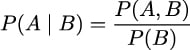
The central panel of Figure 1.8 represents p(A,B) using a grayscale with darker colors for higher probability densities. We see the joint distribution is elongated, indicating that the higher the value of A, the higher the one of B, and vice versa. Knowing the value of A tells us something about the values of B and the other way around. On the top and right margins of Figure 1.8 we have the marginal distributions p(A) and p(B) respectively. To compute the marginal of A, we take p(A,B) and we average overall values of B, intuitively this is like taking a 2D object, the joint distribution, and projecting it into one dimension. The marginal distribution of B is computed similarly. The dashed lines represent the conditional probability p(A|B) for 3 different values of B. We get them by slicing the joint p(A,B) at a given value of B. We can think of this as the distribution of A given that we have observed a particular value of B.
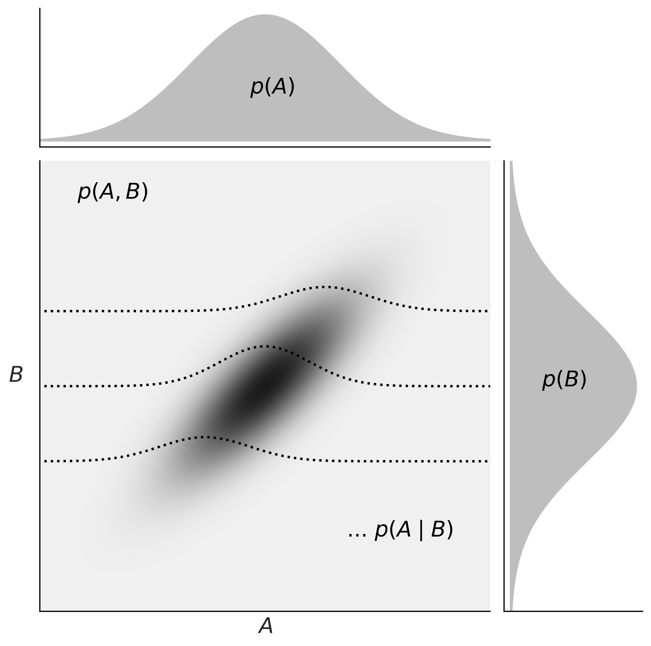
Figure 1.8: Representation of the relationship between the joint p(A,B), the marginals p(A) and p(B), and the conditional p(A|B) probabilities
1.4.7 Expected values
If X is a discrete random variable, we can compute its expected value as:
This is just the mean or average value.
You are probably used to computing means or averages of samples or collections of numbers, either by hand, on a calculator, or using Python. But notice that here we are not talking about the mean of a bunch of numbers; we are talking about the mean of a distribution. Once we have defined the parameters of a distribution, we can, in principle, compute its expected values. Those are properties of the distribution in the same way that the perimeter is a property of a circle that gets defined once we set the value of the radius.
Another expected value is the variance, which we can use to describe the spread of a distribution. The variance appears naturally in many computations in statistics, but in practice, it is often more useful to use the standard deviation, which is the square root of the variance. The reason is that the standard deviation is in the same units as the random variable.
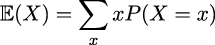
The mean and variance are often called the moments of a distribution. Other moments are skewness, which tells us about the asymmetry of a distribution, and the kurtosis, which tells us about the behavior of the tails or the extreme values [Westfall, 2014]. Figure 1.9 shows examples of different distributions and their mean μ, standard deviation σ, skew γ, and kurtosis  . Notice that for some distributions, some moments may not be defined or they may be inf.
Figure 1.9: Four distributions with their first four moments
Now that we have learned about some of the basic concepts and jargon from probability theory, we can move on to the moment everyone was waiting for.
1.4.8 Bayes’ theorem
Without further ado, let’s contemplate, in all its majesty, Bayes’ theorem:

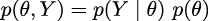
Well, it’s not that impressive, is it? It looks like an elementary school formula, and yet, paraphrasing Richard Feynman, this is all you need to know about Bayesian statistics. Learning where Bayes’ theorem comes from will help us understand its meaning. According to the product rule, we have:

This can also be written as:
Given that the terms on the left are equal for both equations, we can combine them and write:

On reordering, we get Bayes’ theorem:
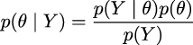
Why is Bayes’ theorem that important? Let’s see.
First, it says that p(θ|Y ) is not necessarily the same as p(Y |θ). This is a very important fact – one that is easy to miss in daily situations, even for people trained in statistics and probability. Let’s use a simple example to clarify why these quantities are not necessarily the same. The probability of a person being the Pope given that this person is Argentinian is not the same as the probability of being Argentinian given that this person is the Pope. As there are around 47,000,000 Argentinians alive and a single one of them is the current Pope, we have p(Pope | Argentinian ) ≈ and we also have p(Argentinian | Pope ) = 1.
If we replace θ with “hypothesis” and Y with “data,” Bayes’ theorem tells us how to compute the probability of a hypothesis, θ, given the data, Y , and that’s the way you will find Bayes’ theorem is explained in a lot of places. But, how do we turn a hypothesis into something that we can put inside Bayes’ theorem? Well, we do it by using probability distributions. So, in general, our hypothesis is a hypothesis in a very, very, very narrow sense; we will be more precise if we talk about finding a suitable value for parameters in our models, that is, parameters of probability distributions. By the way, don’t try to set θ to statements such as ”unicorns are real,” unless you are willing to build a realistic probabilistic model of unicorn existence!
Bayes’ theorem is central to Bayesian statistics. As we will see in Chapter 2, using tools such as PyMC frees us of the need to explicitly write Bayes’ theorem every time we build a Bayesian model. Nevertheless, it is important to know the name of its parts because we will constantly refer to them and it is important to understand what each part means because this will help us to conceptualize models. So, let me rewrite Bayes’ theorem now with labels:
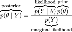
The prior distribution should reflect what we know about the value of the parameter θ before seeing the data, Y . If we know nothing, like Jon Snow, we could use flat priors that do not convey too much information. In general, we can do better than flat priors, as we will learn in this book. The use of priors is why some people still talk about Bayesian statistics as subjective, even when priors are just another assumption that we made when modeling and hence are just as subjective (or objective) as any other assumption, such as likelihoods.
The likelihood is how we will introduce data in our analysis. It is an expression of the plausibility of the data given the parameters. In some texts, you will find people call this term sampling model, statistical model, or just model. We will stick to the name likelihood and we will model the combination of priors and likelihood.
The posterior distribution is the result of the Bayesian analysis and reflects all that we know about a problem (given our data and model). The posterior is a probability distribution for the parameters in our model and not a single value. This distribution is a balance between the prior and the likelihood. There is a well-known joke: a Bayesian is one who, vaguely expecting a horse, and catching a glimpse of a donkey, strongly believes they have seen a mule. One excellent way to kill the mood after hearing this joke is to explain that if the likelihood and priors are both vague, you will get a posterior reflecting vague beliefs about seeing a mule rather than strong ones. Anyway, I like the joke, and I like how it captures the idea of a posterior being somehow a compromise between prior and likelihood. Conceptually, we can think of the posterior as the updated prior in light of (new) data. In theory, the posterior from one analysis can be used as the prior for a new analysis (in practice, life can be harder). This makes Bayesian analysis particularly suitable for analyzing data that becomes available in sequential order. One example could be an early warning system for natural disasters that processes online data coming from meteorological stations and satellites. For more details, read about online machine-learning methods.
The last term is the marginal likelihood, sometimes referred to as the evidence. Formally, the marginal likelihood is the probability of observing the data averaged over all the possible values the parameters can take (as prescribed by the prior). We can write this as ∫ Θp(Y |θ)p(θ)dθ. We will not really care about the marginal likelihood until Chapter 5. But for the moment, we can think of it as a normalization factor that ensures the posterior is a proper pmf or pdf. If we ignore the marginal likelihood, we can write Bayes’ theorem as a proportionality, which is also a common way to write Bayes’ theorem:
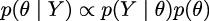
Understanding the exact role of each term in Bayes’ theorem will take some time and practice, and it will require a few examples, but that’s what the rest of this book is for.