Chapter 3
Hierarchical Models

Hierarchical models are one honking great idea – let’s do more of those! - The zen of Bayesian modeling

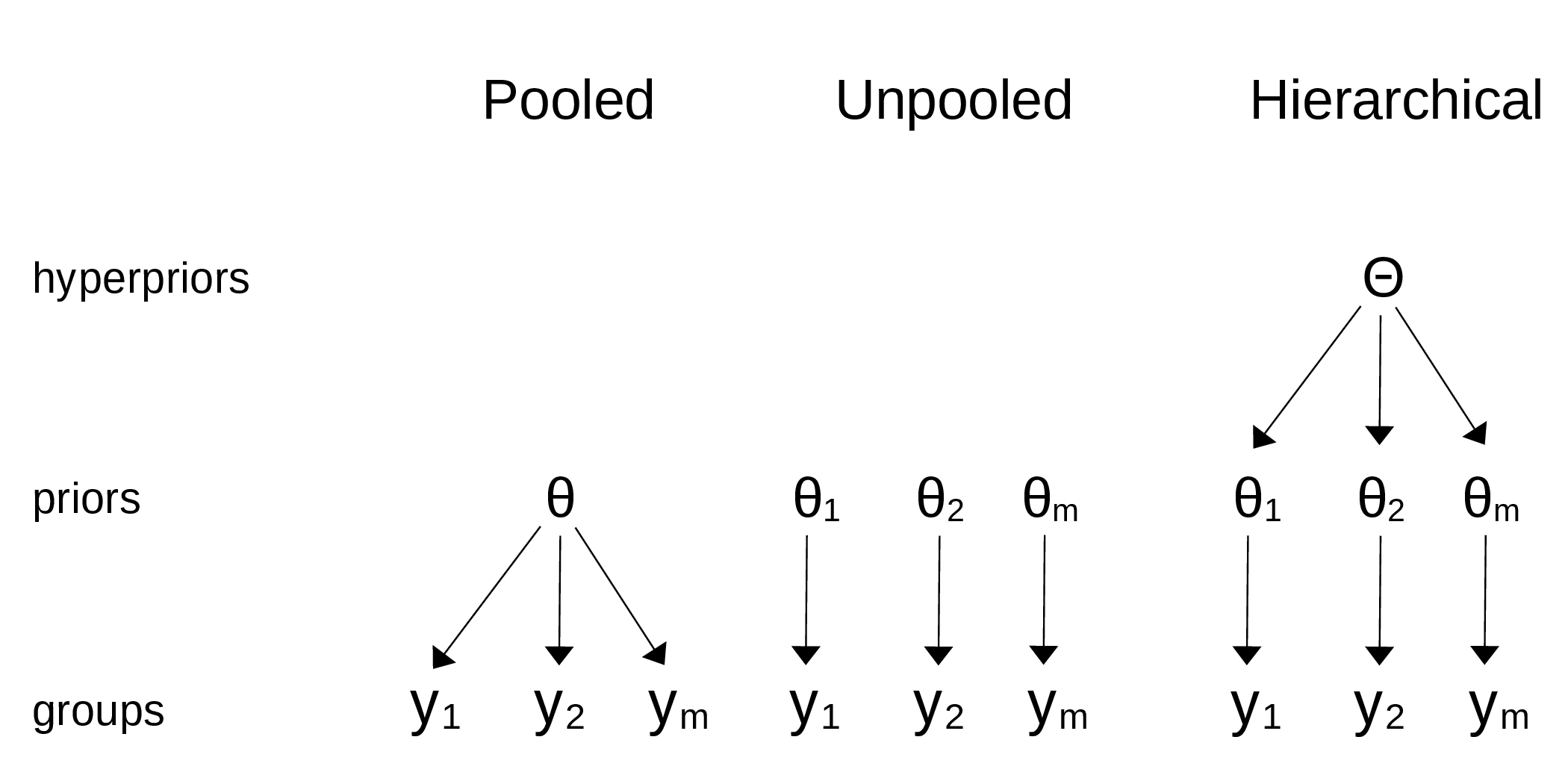
In Chapter 2, we saw a tips example where we had multiple groups in our data, one for each of Thursday, Friday, Saturday, and Sunday. We decided to model each group separately. That’s sometimes fine, but we should be aware of our assumptions. By modeling each group independently, we are assuming the groups are unrelated. In other words, we are assuming that knowing the tip for one day does not give us any information about the tip for another day. That could be too strong an assumption. Would it be possible to build a model that allows us to share information between groups? That’s not only possible, but is also the main topic of this chapter. Lucky you!

In this chapter, we will cover the following topics:

• Hierarchical models

• Partial pooling

• Shrinkage

3.1 Sharing information, sharing priors

Hierarchical models are also known as multilevel models, mixed-effects models, random-effects models, or nested models. They are particularly useful when dealing with data that can be described as grouped or having different levels, such as data nested within geographic regions (for example, cities belonging to a province and provinces belonging to a country), or with a hierarchical structure (such as students nested within schools, or patients nested within hospitals) or repeated measurements on the same individuals.

Figure 3.1: The differences between a pooled model, an unpooled model, and a hierarchical model

Hierarchical models are a natural way to share information between groups. In a hierarchical model, the parameters of the prior distributions are themselves given a prior distribution. These higher-level priors are often called hyperpriors; ”hyper” means ”over” in Greek. Having hyperpriors allows the model...

3.2 Hierarchical shifts

Proteins are molecules formed by 20 units called amino acids. Each amino acid can appear in a protein 0 or more times. Just as a melody is defined by a sequence of musical notes, a protein is defined by a sequence of amino acids. Some musical note variations can result in small variations of the melody and other variations in completely different melodies. Something similar happens with proteins. One way to study proteins is by using nuclear magnetic resonance (the same technique used for medical imaging). This technique allows us to measure various quantities, one of which is called a chemical shift. You may remember that we saw an example using chemical shifts in Chapter 2.

Suppose we want to compare a theoretical method of computing chemical shift against the experimental observations to evaluate the ability of the theoretical method to reproduce the experimental values. Luckily for us, someone has already run the experiments and carried out the theoretical...

3.3 Water quality

Suppose we want to analyze the quality of water in a city, so we take samples by dividing the city into neighborhoods. We may think we have two options for analyzing this data:

• Study each neighborhood as a separate entity

• Pool all the data together and estimate the water quality of the city as a single big group

You have probably already noticed the pattern here. We can justify the first option by saying we obtain a more detailed view of the problem, which otherwise could become invisible or less evident if we average the data. The second option can be justified by saying that if we pool the data, we obtain a bigger sample size and hence a more accurate estimation. But we already know we have a third option: we can do a hierarchical model!

For this example, we are going to use synthetic data. I love using synthetic data; it is a great way to understand things. If you don’t understand something, simulate it! There are many uses for synthetic data. Here, we are...

3.4 Shrinkage

To show you one of the main consequences of hierarchical models, I will require your assistance, so please join me in a brief experiment. I will need you to print and save the summary computed with az.summary(idata_h). Then, I want you to rerun the model two more times after making small changes to the synthetic data. Remember to save the summary after each run. In total, we will have three runs:

• One run setting all the elements of G_samples to 18

• One run setting all the elements of G_samples to 3

• One last run setting one element to 18 and the other two to 3

Before continuing, please take a moment to think about the outcome of this experiment. Focus on the estimated mean value of θ in each experiment. Based on the first two runs of the model, could you predict the outcome for the third case?

If we put the result in a table, we get something more or less like this; remember that small variations could occur due to the stochastic nature of the sampling process:

...

3.5 Hierarchies all the way up

Various data structures lend themselves to hierarchical descriptions that can encompass multiple levels. For example, consider professional football (soccer) players. As in many other sports, players have different positions. We may be interested in estimating some skill metrics for each player, for the positions, and for the overall group of professional football players. This kind of hierarchical structure can be found in many other domains as well:

• Medical research: Suppose we are interested in estimating the effectiveness of different drugs for treating a particular disease. We can categorize patients based on their demographic information, disease severity, and other relevant factors and build a hierarchical model to estimate the probability of cure or treatment success for each subgroup. We can then use the parameters of the subgroup distribution to estimate the overall probability of cure or treatment success for the entire patient population.

• Environmental...

3.6 Summary

In this chapter, we have presented one of the most important concepts to learn from this book: hierarchical models. We can build hierarchical models every time we can identify subgroups in our data. In such cases, instead of treating the subgroups as separate entities or ignoring the subgroups and treating them as a single group, we can build a model to partially pool information among groups. The main effect of this partial pooling is that the estimates of each subgroup will be biased by the estimates of the rest of the subgroups. This effect is known as shrinkage and, in general, is a very useful trick that helps to improve inferences by making them more conservative (as each subgroup informs the others by pulling estimates toward it) and more informative. We get estimates at the subgroup level and the group level.

Paraphrasing the Zen of Python, we can certainly say hierarchical models are one honking great idea, let’s do more of those! In the following chapters...

3.7 Exercises

1. Using your own words explain the following concepts in two or three sentences:

   • Complete pooling

   • No pooling

   • Partial pooling

2. Repeat the exercise we did with model_h. This time, without a hierarchical structure, use a flat prior such as Beta(α = 1,β = 1). Compare the results of both models.

3. Create a hierarchical version of the tips example from Chapter 2, by partially pooling across the days of the week. Compare the results to those obtained without the hierarchical structure.

4. For each subpanel in Figure 3.7, add a reference line representing the empirical mean value at each level, that is, the global mean, the forward mean, and Messi’s mean. Compare the empirical values to the posterior mean values. What do you observe?

5. Amino acids are usually grouped into categories such as polar, non-polar, charged, and special. Build a hierarchical model similar to cs_h but including a group effect for the amino acid category. Compare the results to those...

Join our community Discord space

Join our Discord community to meet like-minded people and learn alongside more than 5000 members at: https://packt.link/bayesian