Chapter 4
Modeling with Lines

In more than three centuries of science everything has changed except perhaps one thing: the love for the simple. – Jorge Wagensberg

Music—from classical compositions to Sheena is a Punk Rocker by The Ramones, passing through unrecognized hits from garage bands and Piazzolla’s Libertango—is made of recurring patterns. The same scales, combinations of chords, riffs, motifs, and so on appear over and over again, giving rise to a wonderful sonic landscape capable of eliciting and modulating the entire range of emotions that humans can experience. Similarly, the universe of statistics is built upon recurring patterns, small motifs that appear now and again. In this chapter, we are going to look at one of the most popular and useful of them, the linear model (or motif, if you want). This is a very useful model on its own and also the building block of many other models. If you’ve ever taken a statistics course, you may...

4.1 Simple linear regression

Many problems we find in science, engineering, and business are of the following form. We have a variable X and we want to model or predict a variable Y . Importantly, these variables are paired like {(x₁,y₁),(x₂,y₂),,(x_n,y_n)}. In the most simple scenario, known as simple linear regression, both X and Y are uni-dimensional continuous random variables. By continuous, we mean a variable represented using real numbers. Using NumPy, you will represent these variables as one-dimensional arrays of floats. Usually, people call Y the dependent, predicted, or outcome variable, and X the independent, predictor, or input variable.

Some typical situations where linear regression models can be used are the following:

• Model the relationship between soil salinity and crop productivity. Then, answer questions such as: is the relationship linear? How strong is this relationship?

• Find a relationship between average chocolate consumption by country and the number of Nobel...

4.2 Linear bikes

We now have a general idea of what Bayesian linear models look like. Let’s try to cement that idea with an example. We are going to start very simply; we have a record of temperatures and the number of bikes rented in a city. We want to model the relationship between the temperature and the number of bikes rented. Figure 4.1 shows a scatter plot of these two variables from the bike-sharing dataset from the UCI Machine Learning Repository ( https://archive.ics.uci.edu/ml/index.php).

Figure 4.1: Bike-sharing dataset. Scatter plot of temperature in Celcius vs. number of rented bikes

The original dataset contains 17,379 records, and each record has 17 variables. We will only use 359 records and two variables, temperature (Celcius) rented (number of rented bikes). We are going to usetemperature as our independent variable (our X) and the number of bikes rented as our dependent variable (our Y). We are going to use the following model:

Code 4.1

with pm...

4.3 Generalizing the linear model

The linear model we have been using is a special case of a more general model, the Generalized Linear Model (GLM). The GLM is a generalization of the linear model that allows us to use different distributions for the likelihood. At a high level, we can write a Bayesian GLM like:

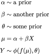
is an arbitrary distribution; some common cases are Normal, Student’s t, Gamma, and NegativeBinomial. θ represents any auxiliary parameter the distribution may have, like σ for the Normal. We also have f, usually called the inverse link function. When is Normal, then f is the identity function. For distributions like Gamma and NegativeBinomial, f is usually the exponential function. Why do we need f? Because the linear model will generally be on the real line, but the μ parameter (or its equivalent) may be defined on a different domain. For instance, μ for the NegativeBinomial is defined for positive values, so we need to transform μ....

4.4 Counting bikes

How can we change model_lb to better accommodate the bike data? There are two things to note: the number of rented bikes is discrete and it is bounded at 0. This is usually known as count data, which is data that is the result of counting something. Count data is sometimes modeled using a continuous distribution like a Normal, especially when the number of counts is large. But it is often a good idea to use a discrete distribution. Two common choices are the Poisson and NegativeBinomial distributions. The main difference is that for Poisson, the mean and the variance are the same, but if this is not true or even approximately true, then NegativeBinomial may be a better choice as it allows the mean and variance to be different. When in doubt, you can fit both Poisson and NegativeBinomial and see which one provides a better model. We are going to do that in Chapter 5. But for now, we are going to use NegativeBinomial.

Code 4.5

with pm.Model() as model_neg: ...

4.5 Robust regression

I once ran a complex simulation of a molecular system. At each step of the simulation, I needed it to fit a linear regression as an intermediate step. I had theoretical and empirical reasons to think that my Y was conditionally Normal given my Xs, so I decided simple linear regression should do the trick. But from time to time the simulation generated a few values of Y that were way above or below the bulk of the data. This completely ruined my simulation and I had to restart it.

Usually, these values that are very different from the bulk of the data are called outliers. The reason for the failure of my simulations was that the outliers were pulling the regression line away from the bulk of the data and when I passed this estimate to the next step in the simulation, the thing just halted. I solved this with the help of our good friend the Student’s t-distribution, which, as we saw in Chapter 2, has heavier tails than the Normal distribution. This means that...

4.6 Logistic regression

The logistic regression model is a generalization of the linear regression model, which we can use when the response variable is binary. This model uses the logistic function as an inverse link function. Let’s get familiar with this function before we move on to the model:

For our purpose, the key property of the logistic function is that irrespective of the values of its argument z, the result will always be a number in the [0-1] interval. Thus, we can see this function as a convenient way to compress the values computed from a linear model into values that we can feed into a Bernoulli distribution. This logistic function is also known as the sigmoid function because of its characteristic S-shaped aspect, as we can see from Figure 4.10.

Figure 4.10: Logistic function

4.6.1 The logistic model

We have almost all the elements to turn a simple linear regression into a simple logistic regression. Let’s begin with the case of only two classes...

4.7 Variable variance

We have been using the linear motif to model the mean of a distribution and, in the previous section, we used it to model interactions. In statistics, it is said that a linear regression model presents heteroskedasticity when the variance of the errors is not constant in all the observations made. For those cases, we may want to consider the variance (or standard deviation) as a (linear) function of the dependent variable.

The World Health Organization and other health institutions around the world collect data for newborns and toddlers and design growth chart standards. These charts are an essential component of the pediatric toolkit and also a measure of the general well-being of populations to formulate health-related policies, plan interventions, and monitor their effectiveness. An example of such data is the lengths (heights) of newborn/toddler girls as a function of their age (in months):

Code 4.9

data = pd.read_csv("data/babies.csv") ...

4.8 Hierarchical linear regression

In Chapter 3, we learned the rudiments of hierarchical models, a very powerful concept that allows us to model complex data structures. Hierarchical models allow us to deal with inferences at the group level and estimations above the group level. As we have already seen, this is done by including hyperpriors. We also showed that groups can share information by using a common hyperprior and this provides shrinkage, which can help us to regularize the estimates.

We can apply these very same concepts to linear regression to obtain hierarchical linear regression models. In this section, we are going to walk through two examples to elucidate the application of these concepts in practical scenarios. The first one uses a synthetic dataset, and the second one uses the pigs dataset.

For the first example, I have created eight related groups, including one group with just one data point. We can see what the data looks like from Figure 4.15. If you want to learn...

4.9 Multiple linear regression

So far, we have been working with one dependent variable and one independent variable. Nevertheless, it is not unusual to have several independent variables that we want to include in our model. Some examples could be:

• Perceived quality of wine (dependent) and acidity, density, alcohol level, residual sugar, and sulfates content (independent variables)

• A student’s average grades (dependent) and family income, distance from home to school, and mother’s education level (categorical variable)

We can easily extend the simple linear regression model to deal with more than one independent variable. We call this model multiple linear regression or, less often, multivariable linear regression (not to be confused with multivariate linear regression, the case where we have multiple dependent variables).

In a multiple linear regression model, we model the mean of the dependent variable as follows:

Using linear algebra notation, we can write a shorter...

4.10 Summary

In this chapter, we have learned about linear regression, which aims to model the relationship between a dependent variable and an independent variable. We have seen how to use PyMC to fit a linear regression model and how to interpret the results and make plots that we can share with different audiences.

Our first example was a model with a Gaussian response. But then we saw that this is just one assumption and we can easily change it to deal with non-Gaussian responses, such as count data, using a NegativeBinomial regression model or a logistic regression model for binary data. We saw that when doing so we also need to set an inverse link function to map the linear predictor to the response variable. Using a Student’s t-distribution as the likelihood can be useful for dealing with outliers. We spent most of the chapter modeling the mean as a linear function of the independent variable, but we learned that we can also model other parameters, like the variance. This...

4.11 Exercises

1. Using the howell dataset (available at https://github.com/aloctavodia/BAP3), create a linear model of the weight (x) against the height (y). Exclude subjects that are younger than 18. Explain the results.

2. For four subjects, we get the weights (45.73, 65.8, 54.2, 32.59), but not their heights. Using the model from the previous exercise, predict the height for each subject, together with their 50% and 94% HDIs. Tip: Use pm.MutableData.

3. Repeat exercise 1, this time including those below 18 years old. Explain the results.

4. It is known for many species that weight does not scale with height, but with the logarithm of the weight. Use this information to fit the howell data (including subjects from all ages).

5. See the accompanying code model_t2 (and the data associated with it). Experiment with priors for ν, like the non-shifted Exponential and Gamma priors (they are commented on in the code). Plot the prior distribution to ensure that you understand them. An easy...

Join our community Discord space

Join our Discord community to meet like-minded people and learn alongside more than 5000 members at: https://packt.link/bayesian