"In God we trust, all others must bring Data"
- Deming
I enjoy working and explaining predictive analytics to people because it is based upon a simple concept: predicting the probability of future events based upon historical data. Its history may date back to at least 650 BC. Some early examples include the Babylonians, who tried to predict short-term weather changes based on cloud appearances and halos: Weather Forecasting through the Ages, NASA.
Medicine also has a long history of needing to classify diseases. The Babylonian king Adad-apla-iddina decreed that medical records be collected to form the Diagnostic Handbook. Some predictions in this corpus list treatments based on the number of days the patient had been sick, and their pulse rate (Linda Miner et al., 2014). One of the first instances of bioinformatics!
In later times, specialized predictive analytics was developed at the onset of the insurance underwriting industries. This was used as a way to predict the risk associated with insuring marine vessels (https://www.lloyds.com/lloyds/about-us/history/corporate-history). At about the same time, life insurance companies began predicting the age that a person would live to in order to set the most appropriate premium rates.
Although the idea of prediction always seemed to be rooted early in the human need to understand and classify, it was not until the 20th century, and the advent of modern computing, that it really took hold.
In addition to helping the US government in the 1940s break code, Alan Turing also worked on the initial computer chess algorithms that pitted man against machine. Monte Carlo simulation methods originated as part of the Manhattan project, where mainframe computers crunched numbers for days in order to determine the probability of nuclear attacks (Computing and the Manhattan Project, n.d).
In the 1950s, Operations Research (OR) theory developed, in which one could optimize the shortest distance between two points. To this day, these techniques are used in logistics by companies such as UPS and Amazon.
Non-mathematicians have also gotten in on the act. In the 1970s, cardiologist Lee Goldman (who worked aboard a submarine) spend years developing a decision tree that did this efficiently. This helped the staff determine whether or not the submarine needed to resurface in order to help the chest pain sufferers (Gladwell, 2005)!
What many of these examples had in common was that people first made observations about events which had already occurred, and then used this information to generalize and then make decisions about might occur in the future. Along with prediction, came further understanding of cause and effect and how the various parts of the problem were interrelated. Discovery and insight came about through methodology and adhering to the scientific method.
Most importantly, they came about in order to find solutions to important, and often practical, problems of the times. That is what made them unique.
We have come a long way since then, and practical analytics solutions have furthered growth in so many different industries. The internet has had a profound effect on this; it has enabled every click to be stored and analyzed. More data is being collected and stored, some with very little effort, than ever before. That in itself has enabled more industries to enter predictive analytics.
One industry that has embraced PA for quite a long time is marketing. Marketing has always been concerned with customer acquisition and retention, and has developed predictive models involving various promotional offers and customer touch points, all geared to keeping customers and acquiring new ones. This is very pronounced in certain segments of marking, such as wireless and online shopping cards, in which customers are always searching for the best deal.
Specifically, advanced analytics can help answer questions such as, If I offer a customer 10% off with free shipping, will that yield more revenue than 15% off with no free shipping? The 360-degree view of the customer has expanded the number of ways one can engage with the customer, therefore enabling marketing mix and attribution modeling to become increasingly important. Location-based devices have enabled marketing predictive applications to incorporate real-time data to issue recommendation to the customer while in the store.
Predictive analytics in healthcare has its roots in clinical trials, which use carefully selected samples to test the efficacy of drugs and treatments. However, healthcare has been going beyond this. With the advent of sensors, data can be incorporated into predictive analytics to monitor patients with critical illness, and to send alerts to the patient when he is at risk. Healthcare companies can now predict which individual patients will comply with courses of treatment advocated by health providers. This will send early warning signs to all parties, which will prevent future complications, as well as lower the total cost of treatment.
Other examples can be found in just about every other industry. Here are just a few:
Although these industries can be quite different, the goals of predictive analytics are typically implemented to increase revenue, decrease costs, or alter outcomes for the better.
So what skills do you need to be successful in predictive analytics? I believe that there are three basic skills that are needed:
Along with the term predictive analytics, here are some terms that are very much related:
Originally, predictive analytics was performed by hand, by statisticians on mainframe computers using a progression of various language such as FORTRAN. Some of these languages are still very much in use today. FORTRAN, for example, is still one of the fastest-performing languages around, and operates with very little memory. So, although it may no longer be as widespread in predictive model development as other languages, it certain can be used to implement models in a production environment.
Nowadays, there are many choices about which software to use, and many loyalists remain true to their chosen software. The reality is that for solving a specific type of predictive analytics problem, there exists a certain amount of overlap, and certainly the goal is the same. Once you get the hang of the methodologies used for predictive analytics in one software package, it should be fairly easy to translate your skills to another package.
Open source emphasizes agile development and community sharing. Of course, open source software is free, but free must also be balanced in the context of Total Cost Of Ownership (TCO). TCO costs include everything that is factored into a softwares cost over a period of time: that not only includes the cost of the software itself, but includes training, infrastructure setup, maintenance, people costs, as well as other expenses associated with the quick upgrade and development cycles which exist in some products.
Closed source (or proprietary) software such as SAS and SPSS was at the forefront of predictive analytics, and has continued to this day to extend its reach beyond the traditional realm of statistics and machine learning. Closed source software emphasizes stability, better support, and security, with better memory management, which are important factors for some companies.
There is much debate nowadays regarding which one is better. My prediction is that they both will coexist peacefully, with one not replacing the other. Data sharing and common APIs will become more common. Each has its place within the data architecture and ecosystem that are deemed correct for a company. Each company will emphasize certain factors, and both open and closed software systems are constantly improving themselves. So, in terms of learning one or the other, it is not an either/or decision. Predictive analytics, per second does not care what software you use. Please be open to the advantages offered by both open and closed software. If you do, that will certainly open up possibilities for working for different kinds of companies and technologies
Man does not live by bread alone, so it would behave you to learn additional tools in addition to R, so as to advance your analytic skills:
sqldf
, which is a popular R package for interfacing with R dataframes. There are other packages that are specifically tailored for the specific database you will be working with.Given that the predictive analytics space is so huge, once you are past the basics, ask yourself what area of predictive analytics really interests you, and what you would like to specialize in. Learning all you can about everything concerning predictive analytics is good at the beginning, but ultimately you will be called upon because you are an expert in certain industries or techniques. This could be research, algorithmic development, or even managing analytics teams.
But, as general guidance, if you are involved in, or are oriented toward, data, the analytics or research portion of data science, I would suggest that you concentrate on data mining methodologies and specific data modeling techniques that are heavily prevalent in the specific industries that interest you.
For example, logistic regression is heavily used in the insurance industry, but social network analysis is not. Economic research is geared toward time series analysis, but not so much cluster analysis. Recommender engines are prevalent in online retail.
If you are involved more on the data engineering side, concentrate more on data cleaning, being able to integrate various data sources, and the tools needed to accomplish this.
If you are a manager, concentrate on model development, testing and control, metadata, and presenting results to upper management in order to demonstrate value or return on investment.
Of course, predictive analytics is becoming more of a team sport, rather than a solo endeavor, and the data science team is very much alive. There is a lot that has been written about the components of a data science team, much of which can be reduced to the three basic skills that I outlined earlier.
Various industries interpret the goals of predictive analytics differently. For example, social science and marketing like to understand the factors which go into a model, and can sacrifice a bit of accuracy if a model can be explained well enough. On the other hand, a black box stock trading model is more interested in minimizing the number of bad trades, and at the end of the day tallies up the gains and losses, not really caring which parts of the trading algorithm worked. Accuracy is more important in the end.
Depending upon how you intend to approach a particular problem, look at how two different analytical mindsets can affect the predictive analytics process:
Of course, the previous examples illustrate two disparate approaches. Combination models, which use the best of both worlds, should be the ones we should strive for. Therefore, one goal for a final model is one which:
You will learn later that is this related to Bias/Variance tradeoff.
Most of the code examples in this book are written in R. As a prerequisite to this book, it is presumed that you will have some basic R knowledge, as well as some exposure to statistics. If you already know about R, you may skip this section, but I wanted to discuss it a little bit for completeness.
The R language is derived from the S language which was developed in the 1970s. However, the R language has grown beyond the original core packages to become an extremely viable environment for predictive analytics.
Although R was developed by statisticians for statisticians, it has come a long way since its early days. The strength of R comes from its package system, which allows specialized or enhanced functionality to be developed and linked to the core system.
Although the original R system was sufficient for statistics and data mining, an important goal of R was to have its system enhanced via user-written contributed packages. At the time of writing, the R system contains more than 10,000 packages. Some are of excellent quality, and some are of dubious quality. Therefore, the goal is to find the truly useful packages that add the most value.
Most, if not all, R packages in use address most common predictive analytics tasks that you will encounter. If you come across a task that does not fit into any category, the chances are good that someone in the R community has done something similar. And of course, there is always a chance that someone is developing a package to do exactly what you want it to do. That person could be eventually be you!
The Comprehensive R Archive Network (CRAN) is a go-to site which aggregates R distributions, binaries, documentation, and packages. To get a sense of the kind of packages that could be valuable to you, check out the Task Views section maintained by CRAN here:
R installation is typically done by downloading the software directly from the Comprehensive R Archive Network (CRAN) site:
Although installing R directly from the CRAN site is the way most people will proceed, I wanted to mention some alternative R installation methods. These methods are often good in instances when you are not always at your computer:
curl
, grep
, awk
, and various customized text editors, such as Emacs Speaks Statistics (ESS). Often R is run this way in production mode, when processes need to be automated and scheduled directly via the operating systemAfter you install R on your own machine, I would give some thought to how you want to organize your data, code, documentation, and so on. There will probably be many different kinds of projects that you will need to set up, ranging from exploratory analysis to full production-grade implementations. However, most projects will be somewhere in the middle, that is, those projects that ask a specific question or a series of related questions. Whatever their purpose, each project you will work on will deserve its own project folder or directory.
Some important points to remember about constructing projects:
subversion
, git
, or cvs
.Once you have considered all of the preceding points, physically set up your folder environment.
We will start by creating folders for our environment. Often projects start with three subfolders which roughly correspond to:
There may be more in certain cases, but lets keep it simple:
PracticalPredictiveAnalytics
. For this example, we will create the directory under Windows drive C.Data
, Outputs
, and R
:
R
directory will hold all of our data prep code, algorithms, and so on.Data
directory will contain our raw data sources that will typically be read in by our programs.Outputs
directory will contain anything generated by the code. That can include plots, tables, listings, and output from the log.Here is an example of how the structure will look after you have created the folders:
R, like many languages and knowledge discovery systems, started from the command line. However, predictive analysts tend to prefer Graphic User Interfaces (GUIs), and there are many choices available for each of the three different operating systems (Mac, Windows, and Linux). Each of them has its strengths and weaknesses, and of course there is always the question of preference.
Memory is always a consideration with R, and if that is of critical concern to you, you might want to go with a simpler GUI, such as the one built in with R.
If you want full control, and you want to add some productive tools, you could choose RStudio, which is a full-blown GUI and allows you to implement version control repositories, and has nice features such as code completion.
R Commander (Rcmdr), and Rattle unique features are that they offer menus that allow guided point and click commands for common statistical and data mining tasks. They are always both code generators. This is a way to start when learning R, since you can use the menus to accomplish the tasks, and then by looking at the way the code was generated for each particular task. If you are interested in predictive analytics using Rattle
, I have written a nice tutorial on using R with Rattle
which can be found in the tutorial section of Practical Predictive Analytics and Decisioning Systems for Medicine, which is referenced at the end of this chapter.
Both RCmdr and RStudio offer GUIs that are compatible with the Windows, Apple, and Linux operator systems, so those are the ones I will use to demonstrate examples in this book. But bear in mind that they are only user interfaces, and not R proper, so it should be easy enough to paste code examples into other GUIs and decide for yourself which ones you like.
After R installation has completed, point your browser to the download section found through the RStudio web site (https://www.rstudio.com/) and install the RStudio executable appropriate for your operating system:
RStudio
icon to bring up the program.
To rearrange the layout, see the following steps:
Tools
| Global Options
| Pane Layout
from the top navigation bar.Environment
| History
| Files
| Plots
and Help
are selected for the upper left paneViewer
is selected for the bottom left pane.Console
for the bottom right paneSource
for the upper right paneOK
.After the changes are applied the layout should more closely match the layout previously shown . However, it may not match exactly. A lot will depend upon the version of RStudio that you are using as well as the packages you may have already installed.
Source
pane will be used to code and save your programs. Once code is created you can use File
| Save
to save your work to an external file, and File |
Open
to retrieve the saved code.If you are installing RStudio for the first time nothing may be shown as the fourth pane. However, as you create new programs (as we will later in this chapter), it will appear in the upper right quadrant.
Console
pane provides important feedback and information about your program after it has been run. It will show you any syntax or error messages that have occurred. It is always a best practice to examine the console to make sure you are getting the results you expect, and make sure the console is clear of errors. The console is also the place that you will see a lots of output which has been created from your programs.View
pane. This pane displays formatted output which is run by using the R View
command.Environment
| History
| Plots
pane is sort of a catch-all pane which changes functions depending upon what which tabs have been selected via the pane layout dialogue. For example, all plots issued by R command are displayed under the Plots
tab. Help is always a click away by selecting the Help
tab. There is also a useful tab called Packages
which will automatically load a package, when a particular package is checked.Once you are set with your layout, proceed to create a new project by following these steps:
Create a new project by following these steps:
File
and then New Project
Existing Directory
:Project working directory
is initial populated with a tilde (~
). This means that the project will be created in the directory you are currently in.Browse
, and then navigate to the PracticalPredictiveAnalytics
folder you created in the previous steps.Choose Directory
dialog box appear, select this directory using the Select Folder
button.Create Project
button. Rstudio will then switch to the new project you have just created.All screen panes will then appear as blank (except for the log), and the title bar at the top left of the screen will show the path to the project.
To verify that the R, outputs, and data directories are contained within the project, select File
, and then File Open
from the top menu bar. The three folders should appear, as indicated as follows:
Once you have verified this, cancel the Open File
dialogue, and return to RStudio main screen.
Now that we have created a project, let us take a look at the R Console window. Click on the window marked Console
. All console commands are issued by typing your command following the command prompt >
, and then pressing Enter. I will just illustrate three commands that will help you answer the questions "Which project am I on?", and "What files do I have in my folders?"
getwd()
: The getwd()
command is very important since it will always tell you which directory you are in. Since we just created a new project, we expect that we will be pointing to the directory we just created, right?
To double check, switch over to the console, issue the getwd()
command, and then press Enter. That should echo back the current working directory:dir()
: The dir()
command will give you a list of all files in the current working directory. In our case, it is simply the names of the three directories you have just created. However, typically may see many files, usually corresponding to the type of directory you are in (.R
for source files, .dat
, .csv
for data files, and so on):setwd()
: Sometimes you will need to switch directories within the same project or even to another project. The command you will use is setwd()
. You will supply the directory that you want to switch to, all contained within the parentheses.
Here is an example which will switch to the sub-directory which will house the R code. This particular example supplies the entire path as the directory destination. Since you are already in the PracticalPredictiveAnalytics
directory, you can also use setwd("R")
which accomplishes the same thing:> setwd("C:/PracticalPredictiveAnalytics/R")
To verify that it has changed, issue the getwd()
command again:
> getwd() [1] "C:/PracticalPredictiveAnalytics/R"
I suggest using getwd()
and setwd()
liberally, especially if you are working on multiple projects, and want to avoid reading or writing the wrong files.
The Source
window is where all of your R code appears. It is also where you will be probably spending most of your time. You can have several script windows open, all at once.
Now that all of the preliminary things are out of the way, we will code our first extremely simple predictive model. There will be two scripts written to accomplish this.
Our first R script is not a predictive model (yet), but it is a preliminary program which will view and plot some data. The dataset we will use is already built into the R package system, and is not necessary to load externally. For quickly illustrating techniques, I will sometimes use sample data contained within specific R packages themselves in order to demonstrate ideas, rather than pulling data in from an external file.
In this case our data will be pulled from the datasets
package, which is loaded by default at startup.
Untitled1
scripts that was just created. Dont worry about what each line means yet. I will cover the specific lines after the code is executed:require(graphics) data(women) head(women) View(women) plot(women$height,women$weight)
Untitled1
tab. It should look something like this:Source
icon. The display should then change to the following diagram:Notice from the preceding picture that three things have changed:
Console
pane.View
pane has popped up which contains a two column table.Plot
pane.Here are some more details on what the code has accomplished:
require
, which is just a way of saying that R needs a specific package to run. In this case require(graphics)
specifies that the graphics
package is needed for the analysis, and it will load it into memory. If it is not available, you will get an error message. However, graphics
is a base package and should be available.Women
data object into memory using the data(women)
function.View(women)
: This will visually display the DataFrame. Although this is part of the actual R script, viewing a DataFrame is a very common task, and is often issued directly as a command via the R Console. As you can see in the previous figure , the Women
dataframe has 15 rows, and 2 columns named height
and weight
.plot(women$height,women$weight)
: This uses the native R plot
function, which plots the values of the two variables against each other. It is usually the first step one does to begin to understand the relationship between two variables. As you can see, the relationship is very linear.head(women)
: This displays the first N rows of the Women
dataframe to the console. If you want no more than a certain number of rows, add that as a second argument of the function. For example, Head(women,99)
will display up to 99 rows in the console. The tail()
function works similarly, but displays the last rows of data.
The utils:View(women)
function can also be shortened to just View(women)
. I have added the prefix utils::
to indicate that the View()
function is part of the utils
package. There is generally no reason to add the prefix unless there is a function name conflict. This can happen when you have identically named functions sourced from two different packages which are loaded in memory. We will see these kind of function name conflicts in later chapters. But it is always safe to prefix a function name with the name of the package that it comes from.
Our second R script is a simple two variable regression model which predicts womens height based upon weight.
Begin by creating another R script by selecting File
| New File
| R Script
from the top navigation bar. If you create new scripts via File
| New File
| R Script
often enough you might get Click Fatigue
(uses three clicks), so you can also save a click by selecting the icon in the top left with the +
sign:
Whichever way you choose , a new blank script window will appear with the name Untitled2
.
Now paste the following code into the new script window:
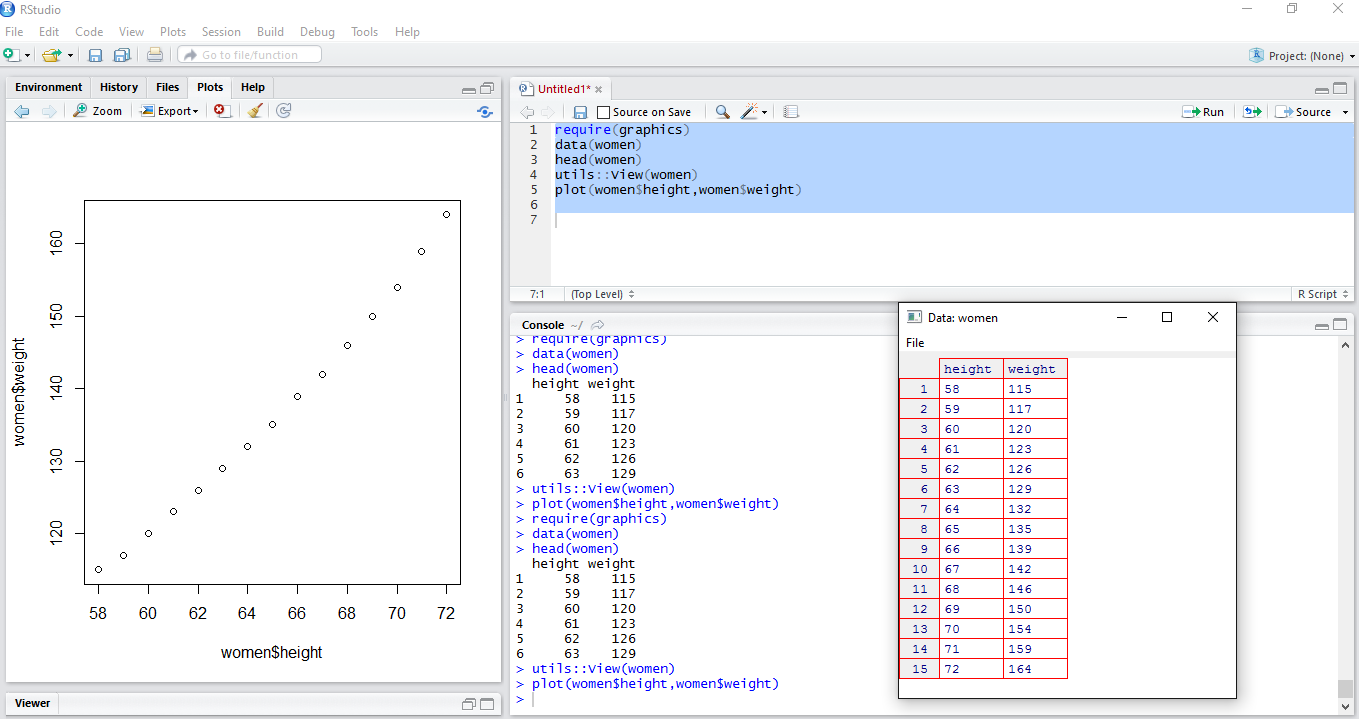
require(graphics) data(women) lm_output <- lm(women$height ~ women$weight) summary(lm_output) prediction <- predict(lm_output) error <- women$height-prediction plot(women$height,error)
Press the Source
icon to run the entire code. The display will change to something similar to what is displayed as follows:
Here are some notes and explanations for the script code that you have just run:
lm()
function: This function runs a simple linear regression using the lm()
function. This function predicts women's height based upon the value of their weight. In statistical parlance, you will be regressing height on weight. The line of code which accomplishes this is:lm_output <- lm(women$height ~ women$weight)
~
operator: Also called the tilde, this is a shorthand way for separating what you want to predict, with what you are using to predict. This is an expression in formula syntax. What you are predicting (the dependent or target variable) is usually on the left side of the formula, and the predictors (independent variables, features) are on the right side. In order to improve readability, the independent variable (weight
) and dependent variable (height
) are specified using $
notation which specifies the object name, $
, and then the dataframe column. So womens height is referenced as women$height
and womens weight is referenced as women$weight.
Alternatively, you can use the attach
command, and then refer to these columns only by specifying the names height
and weight
. For example, the following code would achieve the same results:attach(women) lm_output <- lm(height ~ weight)
<-
operator: Also called the assignment operator. This common statement assigns whatever expressions are evaluated on the right side of the assignment operator to the object specified on the left side of the operator. This will always create or replace a new object that you can further display or manipulate. In this case, we will be creating a new object called lm_output
, which is created using the function lm()
, which creates a linear model based on the formula contained within the parentheses.
Note that the execution of this line does not produce any displayed output. You can see whether the line was executed by checking the console. If there is any problem with running the line (or any line for that matter), you will see an error message in the console.
summary(lm_output)
: The following statement displays some important summary information about the object lm_output
and writes to output to the R Console as pictured previously:summary(lm_output)
Console
window as pictured in the previous figure. Just to keep thing a little bit simpler for now, I will just show the first few lines of the output, and underline what you should be looking at. Do not be discouraged by the amount of output produced.Intercept
and women$weight
which appear under the coefficients line in the console.Coefficients: Estimate Std. Error t value Pr(>|t|) (Intercept) 25.723456 1.043746 24.64 2.68e-12 *** women$weight 0.287249 0.007588 37.85 1.09e-14 ***
Estimate
column illustrates the linear regression formula needed to derive height from weight. We can actually use these numbers along with a calculator to determine the prediction ourselves. For our example the output tells us that we should perform the following steps for all of the observations in our dataframe in order to obtain the prediction for height. We will obviously not want to do all of the observations (R will do that via the following predict()
function), but we will illustrate the calculation for 1 data point:To predict the value for all of the values we will use a function called predict()
. This function reads each input (independent) variable and then predicts a target (dependent) variable based on the linear regression equation. In the code we have assigned the output of this function to a new object named prediction
.
Switch over to the console area, and type prediction
, then Enter, to see the predicted values for the 15 women. The following should appear in the console.
> prediction 1 2 3 4 5 6 7 58.75712 59.33162 60.19336 61.05511 61.91686 62.77861 63.64035 8 9 10 11 12 13 14 64.50210 65.65110 66.51285 67.66184 68.81084 69.95984 71.39608 15 72.83233
Notice that the value of the first prediction is very close to what you just calculated by hand. The difference is due to rounding error.
Another R object produced by our linear regression is the error
object. The error
object is a vector that was computed by taking the difference between the predicted value of height and the actual height. These values are also known as the residual errors, or just residuals.
error <- women$height-prediction
Since the error
object is a vector, you cannot use the nrow()
function to get its size. But you can use the length()
function:
>length(error) [1] 15
In all of the previous cases, the counts all total 15, so all is good. If we want to see the raw data, predictions, and the prediction errors for all of the data, we can use the cbind()
function (Column bind) to concatenate all three of those values, and display as a simple table.
At the console enter the follow cbind
command:
> cbind(height=women$height,PredictedHeight=prediction,ErrorInPrediction=error) height PredictedHeight ErrorInPrediction 1 58 58.75712 -0.75711680 2 59 59.33162 -0.33161526 3 60 60.19336 -0.19336294 4 61 61.05511 -0.05511062 5 62 61.91686 0.08314170 6 63 62.77861 0.22139402 7 64 63.64035 0.35964634 8 65 64.50210 0.49789866 9 66 65.65110 0.34890175 10 67 66.51285 0.48715407 11 68 67.66184 0.33815716 12 69 68.81084 0.18916026 13 70 69.95984 0.04016335 14 71 71.39608 -0.39608278 15 72 72.83233 -0.83232892
From the preceding output, we can see that there are a total 15 predictions. If you compare the ErrorInPrediction
with the error plot shown previously, you can see that for this very simple model, the prediction errors are much larger for extreme values in height (shaded values).
Just to verify that we have one for each of our original observations we will use the nrow()
function to count the number of rows.
At the command prompt in the console area, enter the command:
nrow(women)
The following should appear:
>nrow(women) [1] 15
Refer back to the seventh line of code in the original script: plot(women$height,error)
plots the predicted height versus the errors. It shows how much the prediction was off from the original value. You can see that the errors show a non-random pattern.
After you are done, save the file using File
| File Save
, navigate to the PracticalPredictiveAnalytics/R
folder that was created, and name it Chapter1_LinearRegression
.
An R package extends the functionality of basic R. Base R, by itself, is very capable, and you can do an incredible amount of analytics without adding any additional packages. However adding a package may be beneficial if it adds a functionality which does not exist in base R, improves or builds upon an existing functionality, or just makes something that you can already do easier.
For example, there are no built in packages in base R which enable you to perform certain types of machine learning (such as Random Forests). As a result, you need to search for an add on package which performs this functionality. Fortunately you are covered. There are many packages available which implement this algorithm.
Bear in mind that there are always new packages coming out. I tend to favor packages which have been on CRAN for a long time and have large user base. When installing something new, I will try to reference the results against other packages which do similar things. Speed is another reason to consider adopting a new package.
For an example of a package which can just make life easier, first lets consider the output produced by running a summary function on the regression results, as we did previously. You can run it again if you wish.
summary(lm_output)
The amount of statistical information output by the summary()
function can be overwhelming to the initiated. This is not only related to the amount of output, but the formatting. That is why I did not show the entire output in the previous example.
One way to make output easier to look at is to first reduce the amount of output that is presented, and then reformat it so it is easier on the eyes.
To accomplish this, we can utilize a package called stargazer
, which will reformat the large volume of output produced by summary()
function and simplify the presentations. Stargazer excels at reformatting the output of many regression models, and displaying the results as HTML, PDF, Latex, or as simple formatted text. By default, it will show you the most important statistical output for various models, and you can always specify the types of statistical output that you want to see.
To obtain more information on the stargazer
package you can first go to CRAN, and search for documentation about stargazer
package, and/or you can use the R help system:
IF you already have installed stargazer you can use the following command:
packageDescription("stargazer")
If you havent installed the package, information about stargazer
, (or other packages) can also be found using R specific internet searches:
RSiteSearch("stargazer")
If you like searching for documentation within R, you can obtain more information about the R help system at:
Now, on to installing stargazer:
File
| New File
| R Script
).Source
from the menu bar in the code pane, which will submit the entire script: install.packages("stargazer")
library(stargazer)
stargazer(lm_output, , type="text")
After the script has been run, the following should appear in the Console
:
Here is a line by line description of the code which you have just run:
install.packages("stargazer")
: The line will install the package to the default package directory on your machine. If you will be rerunning this code again, you can comment out this line, since the package will have already be installed in your R repository.library(stargazer)
: Installing a package does not make the package automatically available. You need to run a library (or require()
) function in order to actually load the stargazer
package.
stargazer(lm_output, , type="text")
: This line will take the output object lm_output
, that was created in the first script, condense the output, and write it out to the console in a simpler, more readable format. There are many other options in the stargazer
library, which will format the output as HTML, or Latex.Please refer to the reference manual at https://cran.r-project.org/web/packages/stargazer/index.html for more information.
The reformatted results will appear in the R Console. As you can see, the output written to the console is much cleaner and easier to read.
In this chapter, we have learned a little about what predictive analytics is and how they can be used in various industries. We learned some things about data, and how they can be organized in projects. Finally, we installed RStudio, ran a simple linear regression, and installed and ran our first package. We learned that it is always good practice to examine data after it has been loaded into memory, and a lot can be learned from simply displaying and plotting the data.
In the next chapter, we will discuss the overall predictive modeling process itself, introduce some key model packages using R, and provide some guidance on avoiding some predictive modeling pitfalls.
Where there is an eBook version of a title available, you can buy it from the book details for that title. Add either the standalone eBook or the eBook and print book bundle to your shopping cart. Your eBook will show in your cart as a product on its own. After completing checkout and payment in the normal way, you will receive your receipt on the screen containing a link to a personalised PDF download file. This link will remain active for 30 days. You can download backup copies of the file by logging in to your account at any time.
If you already have Adobe reader installed, then clicking on the link will download and open the PDF file directly. If you don't, then save the PDF file on your machine and download the Reader to view it.
Please Note: Packt eBooks are non-returnable and non-refundable.
Packt eBook and Licensing When you buy an eBook from Packt Publishing, completing your purchase means you accept the terms of our licence agreement. Please read the full text of the agreement. In it we have tried to balance the need for the ebook to be usable for you the reader with our needs to protect the rights of us as Publishers and of our authors. In summary, the agreement says:
If you want to purchase a video course, eBook or Bundle (Print+eBook) please follow below steps:
Our eBooks are currently available in a variety of formats such as PDF and ePubs. In the future, this may well change with trends and development in technology, but please note that our PDFs are not Adobe eBook Reader format, which has greater restrictions on security.
You will need to use Adobe Reader v9 or later in order to read Packt's PDF eBooks.
Packt eBooks are a complete electronic version of the print edition, available in PDF and ePub formats. Every piece of content down to the page numbering is the same. Because we save the costs of printing and shipping the book to you, we are able to offer eBooks at a lower cost than print editions.
When you have purchased an eBook, simply login to your account and click on the link in Your Download Area. We recommend you saving the file to your hard drive before opening it.
For optimal viewing of our eBooks, we recommend you download and install the free Adobe Reader version 9.