


Understanding distributional semantics
Distributional semantics describes the meaning of a word with a vectorial representation, preferably looking at its distributional evidence rather than looking at its predefined dictionary definitions. The theory suggests that words co-occurring together in a similar environment tend to share similar meanings. This was first formulated by the scholar Harris (Distributional Structure Word, 1954). For example, similar words such as dog and cat mostly co-occur in the same context. One of the advantages of a distributional approach is to help the researchers to understand and monitor the semantic evolution of words across time and domains, also known as the lexical semantic change problem.
Traditional approaches have applied Bag-of-Words (BoW) and n-gram language models to build the representation of words and sentences for many years. In a BoW approach, words and documents are represented with a one-hot encoding as a sparse way of representation, also known as the Vector Space Model (VSM).
Text classification, word similarity, semantic relation extraction, word-sense disambiguation, and many other NLP problems have been solved by these one-hot encoding techniques for years. On the other hand, n-gram language models assign probabilities to sequences of words so that we can either compute the probability that a sequence belongs to a corpus or generate a random sequence based on a given corpus.
BoW implementation
A BoW is a representation technique for documents by counting the words in them. The main data structure of the technique is a document-term matrix. Let's see a simple implementation of BoW with Python. The following piece of code illustrates how to build a document-term matrix with the Python sklearn library for a toy corpus of three sentences:
from sklearn.feature_extraction.text import TfidfVectorizer
import numpy as np
import pandas as pd
toy_corpus= ["the fat cat sat on the mat",
             "the big cat slept",
             "the dog chased a cat"]
vectorizer=TfidfVectorizer()
corpus_tfidf=vectorizer.fit_transform(toy_corpus)
print(f"The vocabulary size is \
                 {len(vectorizer.vocabulary_.keys())} ")
print(f"The document-term matrix shape is\
                           {corpus_tfidf.shape}")
df=pd.DataFrame(np.round(corpus_tfidf.toarray(),2))
df.columns=vectorizer.get_feature_names()
The output of the code is a document-term matrix, as shown in the following screenshot. The size is (3 x 10), but in a realistic scenario the matrix size can grow to much larger numbers such as 10K x 10M:
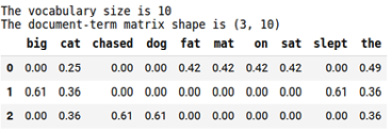
Figure 1.3 – Document-term matrix
The table indicates a count-based mathematical matrix where the cell values are transformed by a Term Frequency-Inverse Document Frequency (TF-IDF) weighting schema. This approach does not care about the position of words. Since the word order strongly determines the meaning, ignoring it leads to a loss of meaning. This is a common problem in a BoW method, which is finally solved by a recursion mechanism in RNN and positional encoding in Transformers.
Each column in the matrix stands for the vector of a word in the vocabulary, and each row stands for the vector of a document. Semantic similarity metrics can be applied to compute the similarity or dissimilarity of the words as well as documents. Most of the time, we use bigrams such as cat_sat and the_street to enrich the document representation. For instance, as the parameter ngram_range=(1,2) is passed to TfidfVectorizer, it builds a vector space containing both unigrams (big, cat, dog) and bigrams (big_cat, big_dog). Thus, such models are also called bag-of-n-grams, which is a natural extension of BoW.
If a word is commonly used in each document, it can be considered to be high-frequency, such as and the. Conversely, some words hardly appear in documents, called low-frequency (or rare) words. As high-frequency and low-frequency words may prevent the model from working properly, TF-IDF, which is one of the most important and well-known weighting mechanisms, is used here as a solution.
Inverse Document Frequency (IDF) is a statistical weight to measure the importance of a word in a document—for example, while the word the has no discriminative power, chased can be highly informative and give clues about the subject of the text. This is because high-frequency words (stopwords, functional words) have little discriminating power in understanding the documents.
The discriminativeness of the terms also depends on the domain—for instance, a list of DL articles is most likely to have the word network in almost every document. IDF can scale down the weights of all terms by using their Document Frequency (DF), where the DF of a word is computed by the number of documents in which a term appears. Term Frequency (TF) is the raw count of a term (word) in a document.
Some of the advantages and disadvantages of a TF-IDF based BoW model are listed as follows:
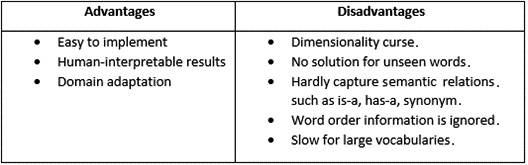
Table 1 – Advantages and disadvantages of a TF-IDF BoW model
Overcoming the dimensionality problem
To overcome the dimensionality problem of the BoW model, Latent Semantic Analysis (LSA) is widely used for capturing semantics in a low-dimensional space. It is a linear method that captures pairwise correlations between terms. LSA-based probabilistic methods can be still considered as a single layer of hidden topic variables. However, current DL models include multiple hidden layers, with billions of parameters. In addition to that, Transformer-based models showed that they can discover latent representations much better than such traditional models.
For the Natural Language Understanding (NLU) tasks, the traditional pipeline starts with some preparation steps, such as tokenization, stemming, noun phrase detection, chunking, stop-word elimination, and much more. Afterward, a document-term matrix is constructed with any weighting schema, where TF-IDF is the most popular one. Finally, the matrix is served as a tabulated input for Machine Learning (ML) pipelines, sentiment analysis, document similarity, document clustering, or measuring the relevancy score between a query and a document. Likewise, terms are represented as a tabular matrix and can be input for a token classification problem where we can apply named-entity recognition, semantic relation extractions, and so on.
The classification phase includes a straightforward implementation of supervised ML algorithms such as Support Vector Machine (SVM), Random forest, logistic, naive bayes, and Multiple Learners (Boosting or Bagging). Practically, the implementation of such a pipeline can simply be coded as follows:
from sklearn.pipeline import make_pipeline
from sklearn.svm import SVC
labels= [0,1,0]
clf = SVC()
clf.fit(df.to_numpy(), labels)
As seen in the preceding code, we can apply fit operations easily thanks to the sklearn Application Programming Interface (API). In order to apply the learned model to train data, the following code is executed:
clf.predict(df.to_numpy())
Output: array([0, 1, 0])
Let's move on to the next section!
Language modeling and generation
For language-generation problems, the traditional approaches are based on leveraging n-gram language models. This is also called a Markov process, which is a stochastic model in which each word (event) depends on a subset of previous words—unigram, bigram, or n-gram, outlined as follows:
- Unigram (all words are independent and no chain): This estimates the probability of word in a vocabulary simply computed by the frequency of it to the total word count.
- Bigram (First-order Markov process): This estimates the P (wordi| wordi-1).probability of wordi depending on wordi-1, which is simply computed by the ratio of P (wordi , wordi-1) to P (wordi-1).
- Ngram (N-order Markov process): This estimates P (wordi | word0, ..., wordi-1).
Let's give a simple language model implementation with the Natural Language Toolkit (NLTK) library. In the following implementation, we train a Maximum Likelihood Estimator (MLE) with order n=2. We can select any n-gram order such as n=1 for unigrams, n=2 for bigrams, n=3 for trigrams, and so forth:
import nltk
from nltk.corpus import gutenberg
from nltk.lm import MLE
from nltk.lm.preprocessing import padded_everygram_pipeline
nltk.download('gutenberg')
nltk.download('punkt')
macbeth = gutenberg.sents('shakespeare-macbeth.txt')
model, vocab = padded_everygram_pipeline(2, macbeth)
lm=MLE(2)
lm.fit(model,vocab)
print(list(lm.vocab)[:10])
print(f"The number of words is {len(lm.vocab)}")
The nltk package first downloads the gutenberg corpus, which includes some texts from the Project Gutenberg electronic text archive, hosted at https://www.gutenberg.org. It also downloads the punkt tokenizer tool for the punctuation process. This tokenizer divides a raw text into a list of sentences by using an unsupervised algorithm. The nltk package already includes a pre-trained English punkt tokenizer model for abbreviation words and collocations. It can be trained on a list of texts in any language before use. In the further chapters, we will discuss how to train different and more efficient tokenizers for Transformer models as well. The following code produces what the language model learned so far:
print(f"The frequency of the term 'Macbeth' is {lm.counts['Macbeth']}")
print(f"The language model probability score of 'Macbeth' is {lm.score('Macbeth')}")
print(f"The number of times 'Macbeth' follows 'Enter' is {lm.counts[['Enter']]['Macbeth']} ")
print(f"P(Macbeth | Enter) is {lm.score('Macbeth', ['Enter'])}")
print(f"P(shaking | for) is {lm.score('shaking', ['for'])}")
This is the output:
The frequency of the term 'Macbeth' is 61
The language model probability score of 'Macbeth' is 0.00226
The number of times 'Macbeth' follows 'Enter' is 15
P(Macbeth | Enter) is 0.1875
P(shaking | for) is 0.0121
The n-gram language model keeps n-gram counts and computes the conditional probability for sentence generation. lm=MLE(2) stands for MLE, which yields the maximum probable sentence from each token probability. The following code produces a random sentence of 10 words with the <s> starting condition given:
lm.generate(10, text_seed=['<s>'], random_seed=42)
The output is shown in the following snippet:
['My', 'Bosome', 'franchis', "'", 's', 'of', 'time', ',', 'We', 'are']
We can give a specific starting condition through the text_seed parameter, which makes the generation be conditioned on the preceding context. In our preceding example, the preceding context is <s>, which is a special token indicating the beginning of a sentence.
So far, we have discussed paradigms underlying traditional NLP models and provided very simple implementations with popular frameworks. We are now moving to the DL section to discuss how neural language models shaped the field of NLP and how neural models overcome the traditional model limitations.