NLP is one of the areas where DL architectures have been widely and successfully used. For decades, we have witnessed successful architectures, especially in word and sentence representation. In this section, we will share the story of these different approaches with commonly used frameworks.
Learning word embeddings
Neural network-based language models effectively solved feature representation and language modeling problems since it became possible to train more complex neural architecture on much larger datasets to build short and dense representations. In 2013, the Word2vec model, which is a popular word-embedding technique, used a simple and effective architecture to learn a high quality of continuous word representations. It outperformed other models for a variety of syntactic and semantic language tasks such as sentiment analysis, paraphrase detection, relation extraction, and so forth. The other key factor in the popularity of the model is its much lower computational complexity. It maximizes the probability of the current word given any surrounding context words, or vice versa.
The following piece of code illustrates how to train word vectors for the sentences of the play Macbeth:
from gensim.models import Word2vec
model = Word2vec(sentences=macbeth, size=100, window= 4, min_count=10, workers=4, iter=10)
The code trains the word embeddings with a vector size of 100 by a sliding 5-length context window. To visualize the words embeddings, we need to reduce the dimension to 3 by applying Principal Component Analysis (PCA) as shown in the following code snippet:
import matplotlib.pyplot as plt
from sklearn.decomposition import PCA
import random
np.random.seed(42)
words=list([e for e in model.wv.vocab if len(e)>4])
random.shuffle(words)
words3d = PCA(n_components=3,random_state=42).fit_transform(model.wv[words[:100]])
def plotWords3D(vecs, words, title):
   ...
plotWords3D(words3d, words, "Visualizing Word2vec Word Embeddings using PCA")
This is the output:
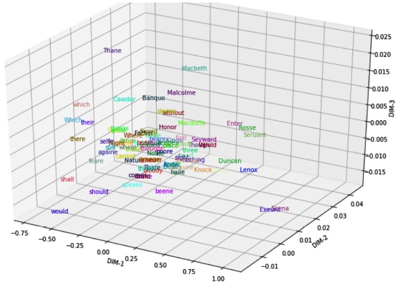
Figure 1.4 – Visualizing word embeddings with PCA
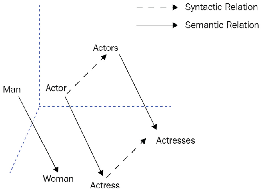
As the plot shows, the main characters of Shakespeare's play—Macbeth, Malcolm, Banquo, Macduff, and others—are mapped close to each other. Likewise, auxiliary verbs shall, should, and would appear close to each other at the left-bottom of Figure 1.4. We can also capture an analogy such as man-woman= uncle-aunt by using an embedding offset. For more interesting visual examples on this topic, please check the following project: https://projector.tensorflow.org/.
The Word2vec-like models learn word embeddings by employing a prediction-based neural architecture. They employ gradient descent on some objective functions and nearby word predictions. While traditional approaches apply a count-based method, neural models design a prediction-based architecture for distributional semantics. Are count-based methods or prediction-based methods the best for distributional word representations? The GloVe approach addressed this problem and argued that these two approaches are not dramatically different. Jeffrey Penington et al. even supported the idea that the count-based methods could be more successful by capturing global statistics. They stated that GloVe outperformed other neural network language models on word analogy, word similarity, and Named Entity Recognition (NER) tasks.
These two paradigms, however, did not provide a helpful solution for unseen words and word-sense problems. They do not exploit subword information, and therefore cannot learn the embeddings of rare and unseen words.
FastText, another widely used model, proposed a new enriched approach using subword information, where each word is represented as a bag of character n-grams. The model sets a constant vector to each character n-gram and represents words as the sum of their sub-vectors, which is an idea that was first introduced by Hinrich Schütze (Word Space, 1993). The model can compute word representations even for unseen words and learn the internal structure of words such as suffixes/affixes, which is especially important with morphologically rich languages such as Finnish, Hungarian, Turkish, Mongolian, Korean, Japanese, Indonesian, and so forth. Currently, modern Transformer architectures use a variety of subword tokenization methods such as WordPiece, SentencePiece, or Byte-Pair Encoding (BPE).
A brief overview of RNNs
RNN models can learn each token representation by rolling up the information of other tokens at an earlier timestep and learn sentence representation at the last timestep. This mechanism has been found beneficial in many ways, outlined as follows:
- Firstly, RNN can be redesigned in a one-to-many model for language generation or music generation.
- Secondly, many-to-one models can be used for text classification or sentiment analysis.
- And lastly, many-to-many models are used for NER problems. The second use of many-to-many models is to solve encoder-decoder problems such as machine translation, question answering, and text summarization.
As with other neural network models, RNN models take tokens produced by a tokenization algorithm that breaks down the entire raw text into atomic units also called tokens. Further, it associates the token units with numeric vectors—token embeddings—which are learned during the training. As an alternative, we can assign the embedded learning task to the well-known word-embedding algorithms such as Word2vec or FastText in advance.
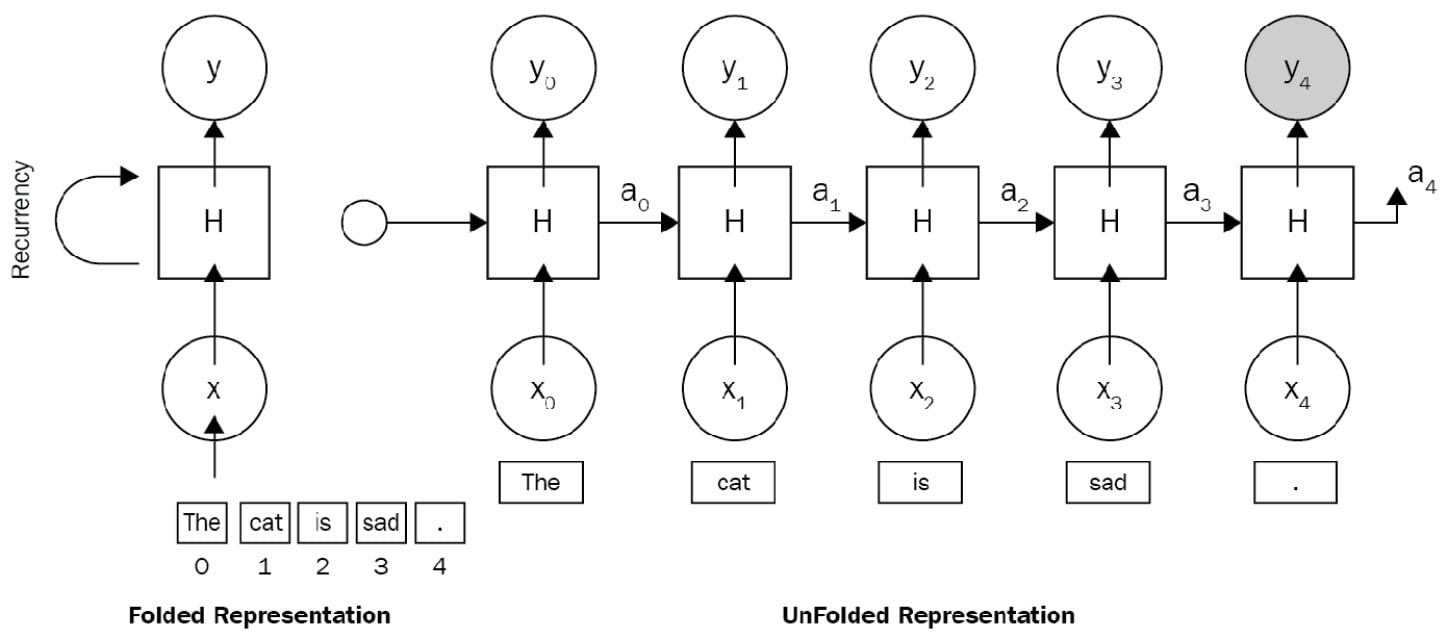
Here is a simple example of an RNN architecture for the sentence The cat is sad., where x0 is the vector embeddings of the, x1 is the vector embeddings of cat, and so forth. Figure 1.5 illustrates an RNN being unfolded into a full Deep Neural Network (DNN).
Unfolding means that we associate a layer to each word. For the The cat is sad. sequence, we take care of a sequence of five words. The hidden state in each layer acts as the memory of the network. It encodes information about what happened in all previous timesteps and in the current timestep. This is represented in the following diagram:
Figure 1.5 – An RNN architecture
The following are some advantages of an RNN architecture:
- Variable-length input: The capacity to work on variable-length input, no matter the size of the sentence being input. We can feed the network with sentences of 3 or 300 words without changing the parameter.
- Caring about word order: It processes the sequence word by word in order, caring about the word position.
- Suitable for working in various modes (many-to-many, one-to-many): We can train a machine translation model or sentiment analysis using the same recurrency paradigm. Both architectures would be based on an RNN.
The disadvantages of an RNN architecture are listed here:
- Long-term dependency problem: When we process a very long document and try to link the terms that are far from each other, we need to care about and encode all irrelevant other terms between these terms.
- Prone to exploding or vanishing gradient problems: When working on long documents, updating the weights of the very first words is a big deal, which makes a model untrainable due to a vanishing gradient problem.
- Hard to apply parallelizable training: Parallelization breaks the main problem down into a smaller problem and executes the solutions at the same time, but RNN follows a classic sequential approach. Each layer strongly depends on previous layers, which makes parallelization impossible.
- The computation is slow as the sequence is long: An RNN could be very efficient for short text problems. It processes longer documents very slowly, besides the long-term dependency problem.
Although an RNN can theoretically attend the information at many timesteps before, in the real world, problems such as long documents and long-term dependencies are impossible to discover. Long sequences are represented within many deep layers. These problems have been addressed by many studies, some of which are outlined here:
- Hochreiter and Schmidhuber. Long Short-term Memory. 1997.
- Bengio et al. Learning long-term dependencies with gradient descent is difficult. 1993.
- K. Cho et al. Learning phrase representations using RNN encoder-decoder for statistical machine translation. 2014.
LSTMs and gated recurrent units
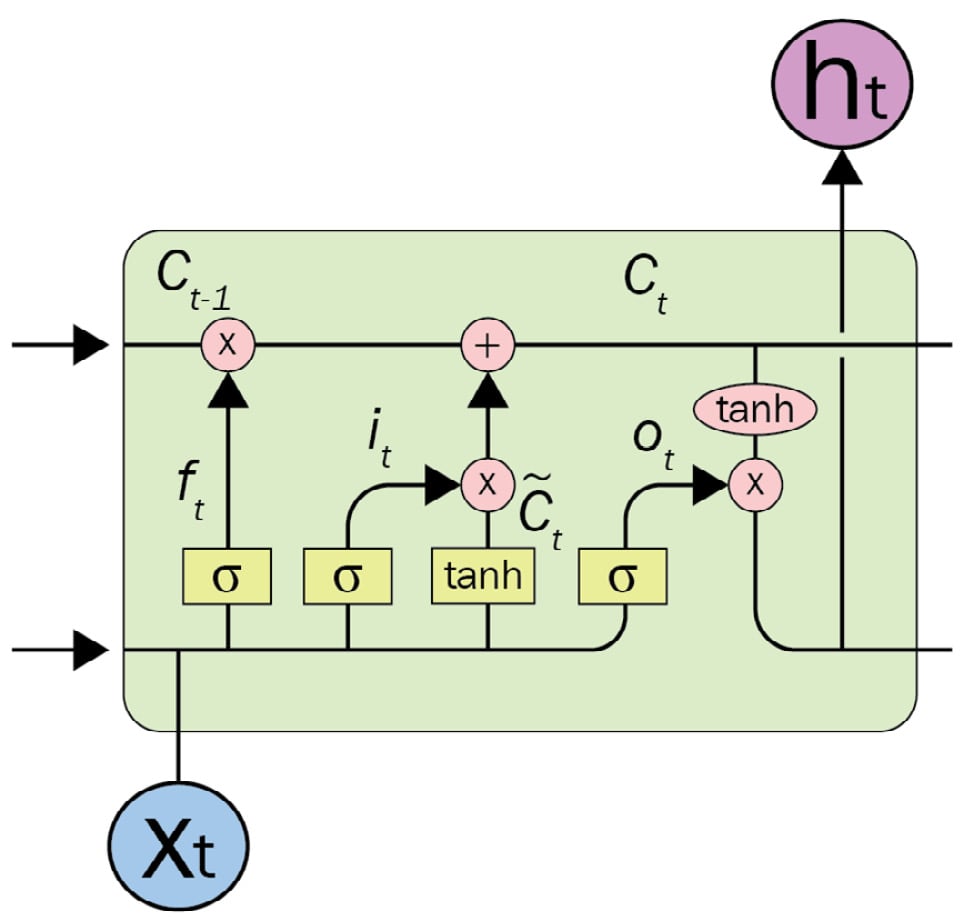
LSTM (Schmidhuber, 1997) and Gated Recurrent Units (GRUs) (Cho, 2014) are new variants of RNNs, have solved long-term dependency problems, and have attracted great attention. LSTMs were particularly developed to cope with the long-term dependency problem. The advantage of an LSTM model is that it uses the additional cell state, which is a horizontal sequence line on the top of the LSTM unit. This cell state is controlled by special purpose gates for forget, insert, or update operations. The complex unit of an LSTM architecture is depicted in the following diagram:
Figure 1.6 – An LSTM unit
It is able to decide the following:
- What kind of information we will store in the cell state
- Which information will be forgotten or deleted
In the original RNN, in order to learn the state of I tokens, it recurrently processes the entire state of previous tokens between timestep0 and timestepi-1. Carrying entire information from earlier timesteps leads to vanishing gradient problems, which makes the model untrainable. The gate mechanism in LSTM allows the architecture to skip some unrelated tokens at a certain timestep or remember long-range states in order to learn the current token state.
A GRU is similar to an LSTM in many ways, the main difference being that a GRU does not use the cell state. Rather, the architecture is simplified by transferring the functionality of the cell state to the hidden state, and it only includes two gates: an update gate and a reset gate. The update gate determines how much information from the previous and current timesteps will be pushed forward. This feature helps the model keep relevant information from the past, which minimizes the risk of a vanishing gradient problem as well. The reset gate detects the irrelevant data and makes the model forget it.
A gentle implementation of LSTM with Keras
We need to download the Stanford Sentiment Treebank (SST-2) sentiment dataset from the General Language Understanding Evaluation (GLUE) benchmark. We can do this by running the following code:
$ wget https://dl.fbaipublicfiles.com/glue/data/SST-2.zip
$ unzip SST-2.zip
Important note
SST-2: This is a fully labeled parse tree that allows for complete sentiment analysis in English. The corpus originally consists of about 12K single sentences extracted from movie reviews. It was parsed with the Stanford parser and includes over 200K unique phrases, each annotated by three human judges. For more information, see Socher et al., Parsing With Compositional Vector Grammars, EMNLP. 2013 (https://nlp.stanford.edu/sentiment).
After downloading the data, let's read it as a pandas object, as follows:
import tensorflow as tf
import pandas as pd
df=pd.read_csv('SST-2/train.tsv',sep="\t")
sentences=df.sentence
labels=df.label
We need to set maximum sentence length, build vocabulary and dictionaries (word2idx, idx2words), and finally represent each sentence as a list of indexes rather than strings. We can do this by running the following code:
max_sen_len=max([len(s.split()) for s in sentences])
words = ["PAD"]+\
     list(set([w for s in sentences for w in s.split()]))
word2idx= {w:i for i,w in enumerate(words)}
max_words=max(word2idx.values())+1
idx2word= {i:w for i,w in enumerate(words)}
train=[list(map(lambda x:word2idx[x], s.split()))\
                                 for s in sentences]
Sequences that are shorter than max_sen_len (maximum sentence length) are padded with a PAD value until they are max_sen_len in length. On the other hand, longer sequences are truncated so that they fit max_sen_len. Here is the implementation:
from keras import preprocessing
train_pad = preprocessing.sequence.pad_sequences(train,
                                    maxlen=max_sen_len)
print('Train shape:', train_pad.shape)
Output: Train shape: (67349, 52)
We are ready to design and train an LSTM model, as follows:
from keras.layers import LSTM, Embedding, Dense
from keras.models import Sequential
model = Sequential()
model.add(Embedding(max_words, 32))
model.add(LSTM(32))
model.add(Dense(1, activation='sigmoid'))
model.compile(optimizer='rmsprop',loss='binary_crossentropy', metrics=['acc'])
history = model.fit(train_pad,labels, epochs=30, batch_size=32, validation_split=0.2)
The model will be trained for 30 epochs. In order to plot what the LSTM model has learned so far, we can execute the following code:
import matplotlib.pyplot as plt
def plot_graphs(history, string):
    ...
plot_graphs(history, 'acc')
plot_graphs(history, 'loss')
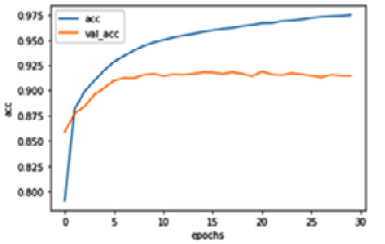
The code produces the following plot, which shows us the training and validation performance of the LSTM-based text classification:
Figure 1.7 – The classification performance of the LSTM network
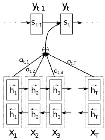
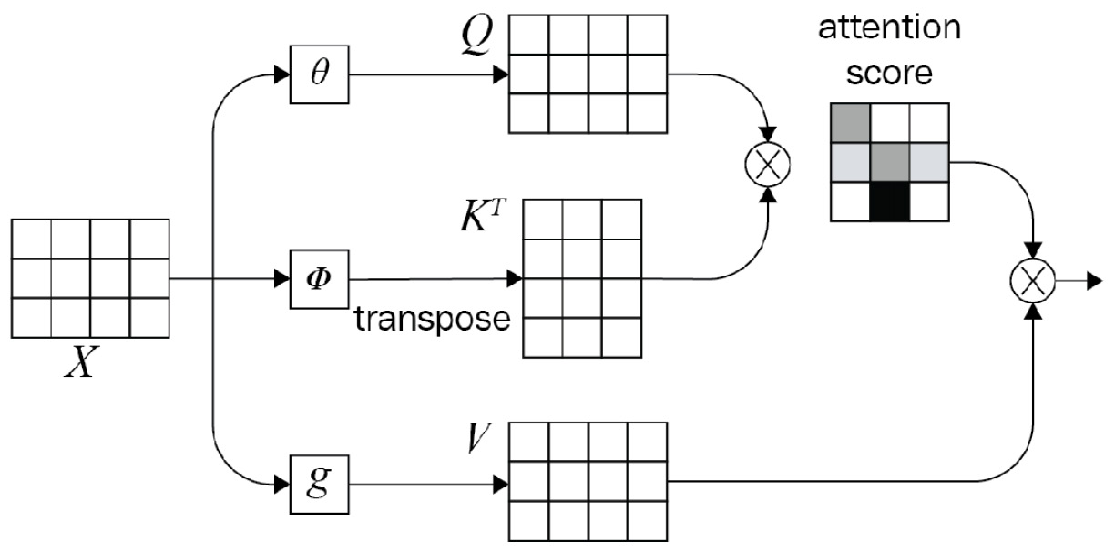
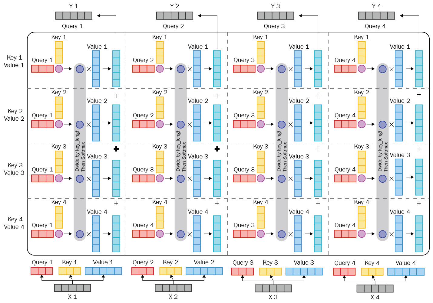
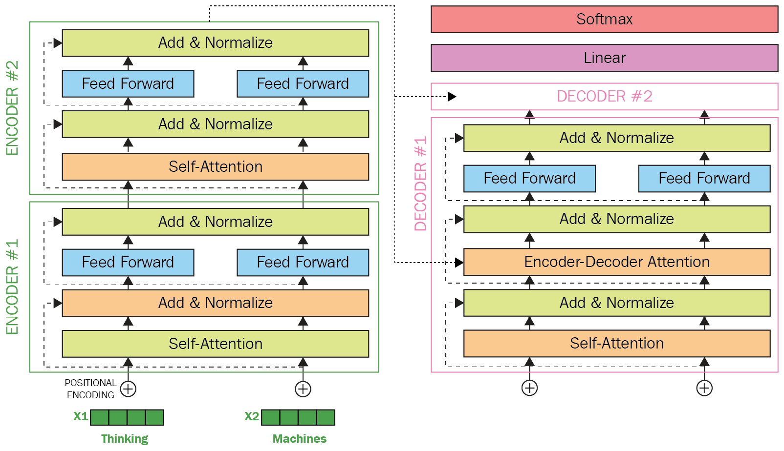
As we mentioned before, the main problem of an RNN-based encoder-decoder model is that it produces a single fixed representation for a sequence. However, the attention mechanism allowed the RNN to focus on certain parts of the input tokens as it maps them to a certain part of the output tokens. This attention mechanism has been found to be useful and has become one of the underlying ideas of the Transformer architecture. We will discuss how the Transformer architecture takes advantage of attention in the next part and throughout the entire book.
A brief overview of CNNs
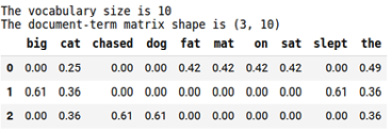
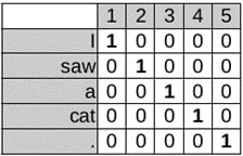
CNNs, after their success in computer vision, were ported to NLP in terms of modeling sentences or tasks such as semantic text classification. A CNN is composed of convolution layers followed by a dense neural network in many practices. A convolution layer performs over the data in order to extract useful features. As with any DL model, a convolution layer plays the feature extraction role to automate feature extraction. This feature layer, in the case of NLP, is fed by an embedding layer that takes sentences as an input in a one-hot vectorized format. The one-hot vectors are generated by a token-id for each word forming a sentence. The left part of the following screenshot shows a one-hot representation of a sentence:
Figure 1.8 – One-hot vectors
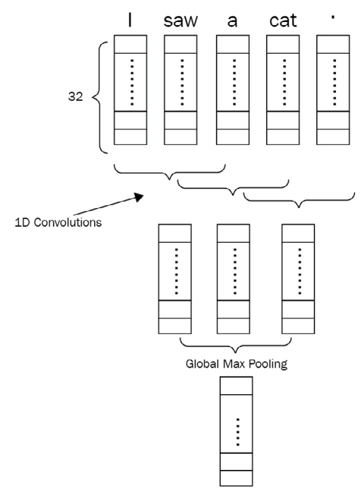
Each token, represented by a one-hot vector, is fed to the embedding layer. The embedding layer can be initialized by random values or by using pre-trained word vectors such as GloVe, Word2vec, or FastText. A sentence will then be transformed into a dense matrix in the shape of NxE (where N is the number of tokens in a sentence and E is the embedding size). The following screenshot illustrates how a 1D CNN processes that dense matrix:
Figure 1.9 – 1D CNN network for a sentence of five tokens
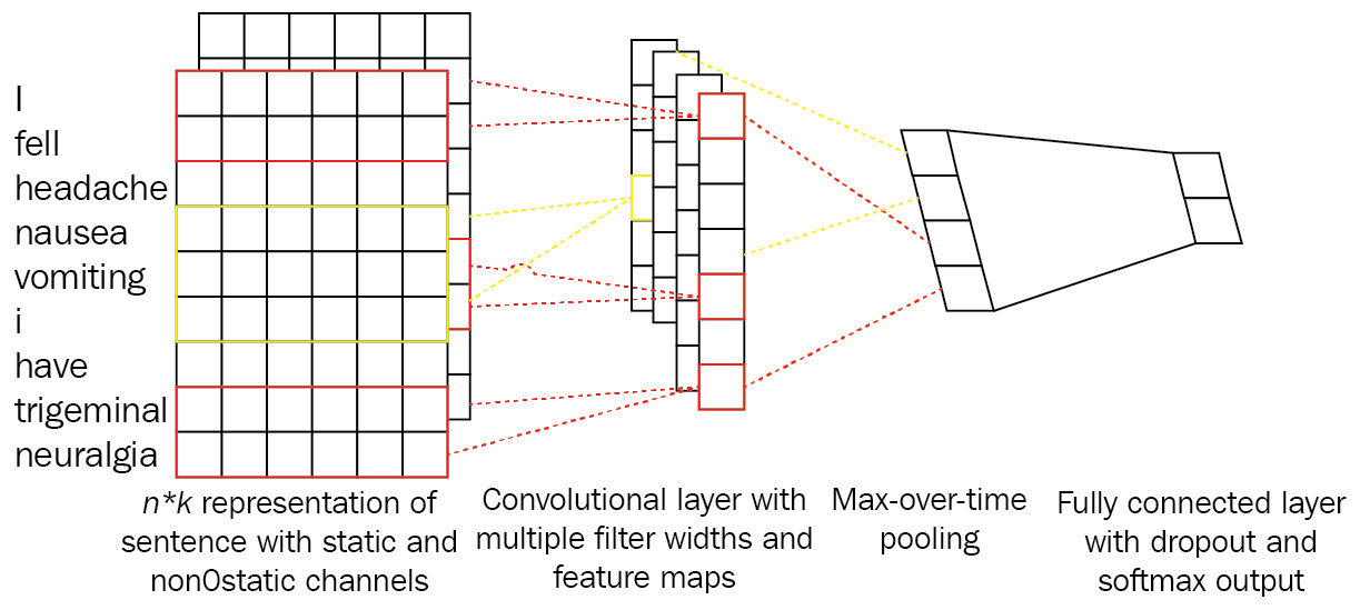
Convolution will take place on top of this operation with different layers and kernels. Hyperparameters for the convolution layer are the kernel size and the number of kernels. It is also good to note that 1D convolution is applied here and the reason for that is token embeddings cannot be seen as partial, and we want to apply kernels capable of seeing multiple tokens in a sequential order together. You can see it as something like an n-gram with a specified window. Using shallow TL combined with CNN models is also another good capability of such models. As shown in the following screenshot, we can also propagate the networks with a combination of many representations of tokens, as proposed in the 2014 study by Yoon Kim, Convolutional Neural Networks for Sentence Classification:
Figure 1.10 – Combination of many representations in a CNN
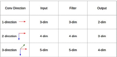
For example, we can use three embedding layers instead of one and concatenate them for each token. Given this setup, a token such as fell will have a vector size of 3x128 if the embedding size is 128 for all three different embeddings. These embeddings can be initialized with pre-trained vectors from Word2vec, GloVe, and FastText. The convolution operation at each step will see N words with their respective three vectors (N is the convolution filter size). The type of convolution that is used here is a 1D convolution. The dimension here denotes possible movements when doing the operation. For example, a 2D convolution will move along two axes, while a 1D convolution just moves along one axis. The following screenshot shows the differences between them:
Figure 1.11 – Convolutional directions
The following code snippet is a 1D CNN implementation processing the same data used in an LSTM pipeline. It includes a composition of Conv1D and MaxPooling layers, followed by GlobalMaxPooling layers. We can extend the pipeline by tweaking the parameters and adding more layers to optimize the model:
from keras import layers
model = Sequential()
model.add(layers.Embedding(max_words, 32, input_length=max_sen_len))
model.add(layers.Conv1D(32, 8, activation='relu'))
model.add(layers.MaxPooling1D(4))
model.add(layers.Conv1D(32, 3, activation='relu'))
model.add(layers.GlobalMaxPooling1D())
model.add(layers.Dense(1, activation= 'sigmoid')
model.compile(loss='binary_crossentropy', metrics=['acc'])
history = model.fit(train_pad,labels, epochs=15, batch_size=32, validation_split=0.2)
It turns out that the CNN model showed comparable performance with its LSTM counterpart. Although CNNs have become a standard in image processing, we have seen many successful applications of CNNs for NLP. While an LSTM model is trained to recognize patterns across time, a CNN model recognizes patterns across space.