Reader small image

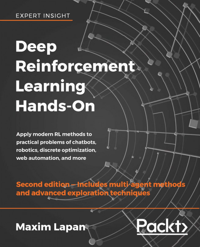
You're reading from  Deep Reinforcement Learning Hands-On. - Second Edition

Product typeBook
Published inJan 2020
Reading LevelIntermediate
PublisherPackt
ISBN-139781838826994
Edition2nd Edition
Languages
Right arrow
Author (1)
Maxim Lapan
Maxim Lapan
author image
Maxim Lapan

Maxim has been working as a software developer for more than 20 years and was involved in various areas: distributed scientific computing, distributed systems and big data processing. Since 2014 he is actively using machine and deep learning to solve practical industrial tasks, such as NLP problems, RL for web crawling and web pages analysis. He has been living in Germany with his family.
Read more about Maxim Lapan

Right arrow

Tabular Learning and the Bellman Equation

In the previous chapter, you became acquainted with your first reinforcement learning (RL) algorithm, the cross-entropy method, along with its strengths and weaknesses. In this new part of the book, we will look at another group of methods that has much more flexibility and power: Q-learning. This chapter will establish the required background shared by those methods.

We will also revisit the FrozenLake environment and explore how new concepts fit with this environment and help us to address issues of its uncertainty.

In this chapter, we will:

  • Review the value of the state and value of the action, and learn how to calculate them in simple cases
  • Talk about the Bellman equation and how it establishes the optimal policy if we know the values
  • Discuss the value iteration method and try it on the FrozenLake environment
  • Do the same for the Q-learning method

Despite the simplicity of the environments in this chapter...
Value, state, and optimality

You may remember our definition of the value of the state from Chapter 1, What Is Reinforcement Learning?. This is a very important notion and the time has come to explore it further.

This whole part of the book is built around the value and how to approximate it. We defined the value as an expected total reward (optionally discounted) that is obtainable from the state. In a formal way, the value of the state is , where rt is the local reward obtained at step t of the episode.

The total reward could be discounted with or not (the undiscounted case corresponds to ); it's up to us how to define it. The value is always calculated in terms of some policy that our agent follows. To illustrate this, let's consider a very simple environment with three states:

  1. The agent's initial state.
  2. The final state that the agent is in after executing action "right" from the initial state. The reward obtained from this is 1.
  3. ...

The Bellman equation of optimality

To explain the Bellman equation, it's better to go a bit abstract. Don't be afraid; I'll provide concrete examples later to support your learning! Let's start with a deterministic case, when all our actions have a 100% guaranteed outcome. Imagine that our agent observes state s0 and has N available actions. Every action leads to another state, s1 ... sN, with a respective reward, r1 ... rN. Also, assume that we know the values, Vi, of all states connected to state s0. What will be the best course of action that the agent can take in such a state?

Figure 5.3: An abstract environment with N states reachable from the initial state

If we choose the concrete action, ai, and calculate the value given to this action, then the value will be . So, to choose the best possible action, the agent needs to calculate the resulting values for every action and choose the maximum possible outcome. In other words, . If we are using the...

The value of the action

To make our life slightly easier, we can define different quantities, in addition to the value of the state, V(s), as the value of the action, Q(s, a). Basically, this equals the total reward we can get by executing action a in state s and can be defined via V(s). Being a much less fundamental entity than V(s), this quantity gave a name to the whole family of methods called Q-learning, because it is more convenient.

In these methods, our primary objective is to get values of Q for every pair of state and action.

Q for this state, s, and action, a, equals the expected immediate reward and the discounted long-term reward of the destination state. We also can define V(s) via Q(s, a):

This just means that the value of some state equals to the value of the maximum action we can execute from this state. Finally, we can express Q(s, a) recursively (which will be used in Chapter 6, Deep Q-Networks:

In the preceding formula, the index on the...

The value iteration method

In the simplistic example you just saw, to calculate the values of the states and actions, we exploited the structure of the environment: we had no loops in transitions, so we could start from terminal states, calculate their values, and then proceed to the central state. However, just one loop in the environment builds an obstacle in our approach. Let's consider such an environment with two states:

Figure 5.7: A sample environment with a loop in the transition diagram

We start from state s1, and the only action we can take leads us to state s2. We get the reward r = 1, and the only transition from s2 is an action, which brings us back to s1. So, the life of our agent is an infinite sequence of states . To deal with this infinity loop, we can use a discount factor: . Now, the question is, what are the values for both the states? The answer is not very complicated, in fact. Every transition from s1 to s2 gives us a reward of 1 and every back...

Value iteration in practice

The complete example is in Chapter05/01_frozenlake_v_iteration.py. The central data structures in this example are as follows:

  • Reward table: A dictionary with the composite key "source state" + "action" + "target state". The value is obtained from the immediate reward.
  • Transitions table: A dictionary keeping counters of the experienced transitions. The key is the composite "state" + "action", and the value is another dictionary that maps the target state into a count of times that we have seen it. For example, if in state 0 we execute action 1 ten times, after three times it will lead us to state 4 and after seven times to state 5.

    The entry with the key (0, 1) in this table will be a dict with contents {4: 3, 5: 7}. We can use this table to estimate the probabilities of our transitions.

  • Value table: A dictionary that maps a state into the calculated value of this state.

The overall...

Q-learning for FrozenLake

The whole example is in the Chapter05/02_frozenlake_q_iteration.py file, and the difference is really minor. The most obvious change is to our value table. In the previous example, we kept the value of the state, so the key in the dictionary was just a state. Now we need to store values of the Q-function, which has two parameters: state and action, so the key in the value table is now a composite.

The second difference is in our calc_action_value() function. We just don't need it anymore, as our action values are stored in the value table.

Finally, the most important change in the code is in the agent's value_iteration() method. Before, it was just a wrapper around the calc_action_value() call, which did the job of Bellman approximation. Now, as this function has gone and been replaced by a value table, we need to do this approximation in the value_iteration() method.

Let's look at the code. As it's almost the same, I will jump...

Summary

My congratulations, you have made another step towards understanding modern, state-of-the-art RL methods! In this chapter, you learned about some very important concepts that are widely used in deep RL: the value of the state, the value of the action, and the Bellman equation in various forms.

We also covered the value iteration method, which is a very important building block in the area of Q-learning. Finally, you got to know how value iteration can improve our FrozenLake solution.

In the next chapter, you will learn about deep Q-networks, which started the deep RL revolution in 2013 by beating humans on lots of Atari 2600 games.

lock icon
The rest of the chapter is locked
You have been reading a chapter from
Deep Reinforcement Learning Hands-On. - Second Edition
Published in: Jan 2020Publisher: PacktISBN-13: 9781838826994
Register for a free Packt account to unlock a world of extra content!
A free Packt account unlocks extra newsletters, articles, discounted offers, and much more. Start advancing your knowledge today.
undefined
Unlock this book and the full library FREE for 7 days
Get unlimited access to 7000+ expert-authored eBooks and videos courses covering every tech area you can think of
Renews at €14.99/month. Cancel anytime

Author (1)

author image
Maxim Lapan

Maxim has been working as a software developer for more than 20 years and was involved in various areas: distributed scientific computing, distributed systems and big data processing. Since 2014 he is actively using machine and deep learning to solve practical industrial tasks, such as NLP problems, RL for web crawling and web pages analysis. He has been living in Germany with his family.
Read more about Maxim Lapan