Reader small image

You're reading from  Scientific Computing with Python 3

Product typeBook
Published inDec 2016
Reading LevelBeginner
PublisherPackt
ISBN-139781786463517
Edition1st Edition
Languages
Right arrow
Authors (3):
Claus Führer
Claus Führer
author image
Claus Führer

Claus Führer is a professor of scientific computations at Lund University, Sweden. He has an extensive teaching record that includes intensive programming courses in numerical analysis and engineering mathematics across various levels in many different countries and teaching environments. Claus also develops numerical software in research collaboration with industry and received Lund University's Faculty of Engineering Best Teacher Award in 2016.
Read more about Claus Führer

View More author details
Right arrow

Chapter 4. Linear Algebra – Arrays

Linear algebra is one of the essential building blocks of computational mathematics. The objects of linear algebra are vectors and matrices. The package NumPy includes all the necessary tools to manipulate those objects.

The first task is to build matrices and vectors, or to alter existing ones by slicing. The other main task is the dot operation, which embodies most of the linear algebra operations (scalar product, matrix-vector product, and matrix-matrix product). Finally, various methods are available to solve linear problems.

Overview of the array type


For the impatient, here is how to use arrays in a nutshell. Be aware though that the behavior of arrays may be surprising at first, so we encourage you to read on after this introductory section.

Vectors and matrices

Creating vectors is as simple as using the function array  to convert a list to an array:

v = array([1.,2.,3.])

The object v  is now a vector that behaves much like a vector in linear algebra. We have already emphasized the differences with the list object in Python (refer to section Arrays in Chapter 3, Containers Type). Here are some illustrations of the basic linear algebra operations on vectors:

# two vectors with three components
v1 = array([1., 2., 3.])
v2 = array([2, 0, 1.])

# scalar multiplications/divisions
2*v1 # array([2., 4., 6.])
v1/2 # array([0.5, 1., 1.5])

# linear combinations
3*v1 # array([ 3., 6., 9.])
3*v1 + 2*v2 # array([ 7., 6., 11.])

# norm
from scipy.linalg import...

Mathematical preliminaries


In order to understand how arrays work in NumPy, it is useful to understand the mathematical parallel between accessing tensor (matrix and vector) elements by indexes and evaluating mathematical functions by providing arguments. We also cover in this section the generalization of the dot product as a reduction operator.

Arrays as functions

Arrays may be considered from several different points of view. We believe that the most fruitful one in order to understand arrays is that of functions of several variables.

For instance, selecting a component of a given vector in n may just be considered a function from the set of ℕn to ℝ, where we define the set:

Here the set ℕn has n elements. The Python function range generates ℕn.

Selecting an element of a given matrix, on the other hand, is a function of two parameters, taking its value in ℝ. Picking a particular element of an m × n matrix may thus be considered a function from ℕm × ℕn to ℝ.

Operations are elementwise

NumPy...

The array type


The objects used to manipulate vectors, matrices, and more general tensors in NumPy are called arrays. In this section, we examine their essential properties, how to create them, and how to access their information.

Array properties

Arrays are essentially characterized by three properties, which is given in the following table (Table 4.2):

Accessing array entries


Array entries are accessed by indexes. In contrast to vector coefficients two indexes are needed to access matrix coefficients. These are given in one pair of brackets. This distinguishes the array syntax from a list of lists. There, two pairs of brackets are needed to access elements.

M = array([[1., 2.],[3., 4.]])
M[0, 0] # first row, first column: 1.
M[-1, 0] # last row, first column: 3.

Basic array slicing

Slices are similar to those of lists except that there might now be in more than one dimension:

  • M[i,:] is a vector filled by the row i of M.
  • M[:,j] is a vector filled by the column i of M.
  • M[2:4,:] is a slice of 2:4 on the rows only.
  • M[2:4,1:4] is a slice on rows and columns.

The result of matrix slicing is given in the following figure (Figure 4.1):

Figure 4.1: The result of matrix slicing

Note

Omitting a dimension

If you omit an index or a slice, NumPy assumes you are taking rows only. M[3] is a vector that is a view on the third row of and M[1:3] is a...

Functions to construct arrays


The usual way to set up an array is via a list. But there are also a couple of convenient methods for generating special arrays, which are given in the following table (Table 4.5):

Name

Description

shape

It describes how the data should be interpreted, as a vector, a matrix or as a higher order tensor, and it gives the corresponding dimension. It is accessed with the shape attribute.

dtype

It gives the type of the underlying data (float, complex, integer, and so on).

strides

This attribute specifies in which order the data should be read. For instance, a matrix could be stored in memory contiguously column by column (the FORTRAN convention), or row by row (the C convention). The attribute is a tuple with the numbers of bytes that have to be skipped in memory to reach the next row and the number of bytes...

Methods

Shape

Generates

 zeros((n,m))

(n,m)

Matrix filled with zeros

ones((n,m)) 

(n,m)

Matrix filled with ones

diag(v,k) 

(n,n)

(Sub-, super-) diagonal matrix from a vector v

random.rand(n,m) 

(n,m)

Matrix filled with uniformly distributed random numbers in (0,1)

 arange(n)

(n,)

First n integers

linspace(a,b,n) 

(n,)

Vector with n equispaced points between a and b

Table 4.5: Commands to create arrays

These commands may take additional arguments. In particular, the commands zeros, ones, and arange take dtype as an optional argument. The default type is float, except for arange. There are also methods such as zeros_like and ones_like, which are slight variants of the preceding ones. For instance, the zeros_like(A) method is equivalent...

Accessing and changing the shape


The number of dimensions is what distinguishes a vector from a matrix. The shape is what distinguishes vectors of different sizes, or matrices of different sizes. In this section, we examine how to obtain and change the shape of an array.

The shape function

The shape of a matrix is the tuple of its dimensions. The shape of an n × m matrix is the tuple (n, m). It can be obtained by the shape function:

M = identity(3)
shape(M) # (3, 3)

For a vector, the shape is a singleton containing the length of that vector:

v = array([1., 2., 1., 4.])
shape(v) # (4,) <- singleton (1-tuple)

An alternative is to use the array attribute shape, which gives  the same result:

M = array([[1.,2.]])
shape(M) # (1,2)
M.shape # (1,2)

However, the advantage of using  shape as a function is that this function may be used on scalars and lists as well. This may come in handy when code is supposed to work with both scalars and arrays:

shape(1.) # ()
shape([1,2]) # (2...

Stacking


The universal method to build matrices from a couple of (matching) submatrices is concatenate. Its syntax is:

concatenate((a1, a2, ...), axis = 0)

This command stacks the submatrices vertically (on top of each other) when axis=0 is specified. With the axis=1 argument, they are stacked horizontally, and this generalizes according to arrays with more dimensions. This function is called by several convenient functions, as follows:

  • hstack: Used to stack matrices horizontally
  • vstack: Used to stack matrices vertically
  • columnstack: Used to stack vectors in columns

Stacking vectors

One may stack vectors row-wise or column-wise using vstack and column_stack, as illustrated in the following figure:

Tip

hstack would produce the concatenation of v1 and v2. 

Let us consider the symplectic permutation as an example for vector stacking: We have a vector of size 2n. We want to perform a symplectic transformation of a vector with an even number of components, that is, exchange the first half with the second...

Functions acting on arrays


There are different types of functions acting on arrays. Some act elementwise, and they return an array of the same shape. Those are called universal functions. Other array functions return an array of a different shape.

Universal functions

Universal functions are functions that act elementwise on arrays. They thus have an output array that has the same shape as the input array. These functions allow us to compute the result of a scalar function on a whole array at once.

Built-in universal functions

A typical example is the cos function (the one provided by NumPy):

cos(pi) # -1
cos(array([[0, pi/2, pi]])) # array([[1, 0, -1]])

Note that universal functions work on arrays in a componentwise manner. This is also true for operators, such as multiplication or exponent:

2 * array([2, 4]) # array([4, 8])
array([1, 2]) * array([1, 8]) # array([1, 16])
array([1, 2])**2 # array([1, 4])
2**array([1, 2]) # array([1, 4])
array([1, 2])**array([1, 2]) # array...

Linear algebra methods in SciPy


SciPy offers a large range of methods from numerical linear algebra in its scipy.linalg module. Many of these methods are Python wrapping programs from LAPACK, a collection of well-approved FORTRAN subroutines used to solve linear equation systems and eigenvalue problems. Linear algebra methods are the core of any method in scientific computing, and the fact that SciPy uses wrappers instead of pure Python code makes these central methods extremely fast. We present in detail here how two linear algebra problems are solved with SciPy to give you a flavour of this module.

Solving several linear equation systems with LU

Let A be an n × n matrix and b1 , b2 , ..., bk  be a sequence of n-vectors. We consider the problem to find n vectors xi such that:

We assume that the vectors bi are not known simultaneously. In particular, it is quite a common situation that the ith problem has to be solved before bi+1 becomes available.

LU factorization is a way to organize...

Summary


In this chapter, we worked with the most important objects in linear algebra – vectors and matrices. For this, we learned how to define arrays and we met important array methods. A smaller section demonstrated how to use modules from scipy.linalg to solve central tasks in linear algebra.

Exercises


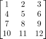
Ex. 1 → Consider a 4 × 3 matrix M:

  1. Construct this matrix in Python using the function array .
  2. Construct the same matrix using the function arange  followed by a suitable reshape.
  3. What is the result of the expression M[2,:] ? What is the result of the similar expression M[2:]?

Ex. 2 → Given a vector x, construct in Python the following matrix:


Here, xi are the components of the vector x (numbered from zero). Given a vector y, solve in Python the linear equation system Va = y. Let the components of a be denoted by ai, i = 0, ..., 5. Write a function poly, which has a and z as input and which computes the polynomial:

Plot this polynomial and depict in the same plot the points (xi , yi ) as small stars. Try your code with the vectors:

  • x = (0.0, 0.5, 1.o, 1.5, 2.0, 2.5)
  • y = (-2.0, 0.5, -2.0, 1.0, -0.5, 1.0)

Ex. 3 → The matrix V in Ex. 2 is called a Vandermonde matrix. It can be set up in Python directly by the command vander. Evaluating a polynomial defined by a coefficient...

lock icon
The rest of the chapter is locked
You have been reading a chapter from
Scientific Computing with Python 3
Published in: Dec 2016Publisher: PacktISBN-13: 9781786463517
Register for a free Packt account to unlock a world of extra content!
A free Packt account unlocks extra newsletters, articles, discounted offers, and much more. Start advancing your knowledge today.
undefined
Unlock this book and the full library FREE for 7 days
Get unlimited access to 7000+ expert-authored eBooks and videos courses covering every tech area you can think of
Renews at AU $19.99/month. Cancel anytime

Authors (3)

author image
Claus Führer

Claus Führer is a professor of scientific computations at Lund University, Sweden. He has an extensive teaching record that includes intensive programming courses in numerical analysis and engineering mathematics across various levels in many different countries and teaching environments. Claus also develops numerical software in research collaboration with industry and received Lund University's Faculty of Engineering Best Teacher Award in 2016.
Read more about Claus Führer