Plotting in Python can be done with the pyplot part of the matplotlib module. With matplotlib you can create high-quality figures and graphics and also plot and visualize your results. Matplotlib is open source and freely available software, [21]. The matplotlib website also contains excellent documentation with examples, [35]. In this section, we will show you how to use the most common features. The examples in the upcoming sections assume that you have imported the module as:
from matplotlib.pyplot import *
In case you want to use the plotting commands in IPython, it is recommended that you run the magic command %matplotlib directly after starting the IPython shell. This prepares IPython for interactive plotting.
The standard plotting function is plot. Calling plot(x,y) creates a figure window with a plot of y as a function of x. The input arguments are arrays (or lists) of equal length. It is also possible to use plot(y), in which case the values in y will be plotted against their index, that is, plot(y) is a short form of plot(range(len(y)),y).
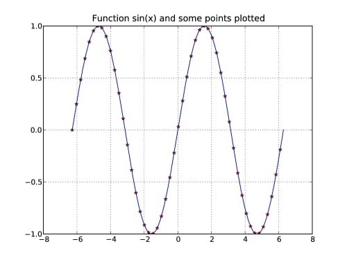
Here is an example that shows how to plot sin(x) for x ϵ [-2π, 2π] using 200 sample points and sets markers at every fourth point:
# plot sin(x) for some interval
x = linspace(-2*pi,2*pi,200)
plot(x,sin(x))

# plot marker for every 4th point
samples = x[::4]
plot(samples,sin(samples),'r*')

# add title and grid lines
title('Function sin(x) and some points plotted')
grid()
The result is shown in the following figure (Figure 6.1):
Figure 6.1: A plot of the function sin(x) with grid lines shown.
As you can see, the standard plot is a solid blue curve. Each axis gets automatically scaled to fit...
The appearance of figures and plots can be styled and customized to look how you want them to look. Some important variables are linewidth, which controls the thickness of plot lines; xlabel, ylabel, which set the axis labels, color for plot colors, and transparent for transparency. This section will tell you how to use some of them. The following is an example with more keywords:
k = 0.2
x = [sin(2*n*k) for n in range(20)]
plot(x, color='green', linestyle='dashed', marker='o',
                       markerfacecolor='blue', markersize=12, linewidth=6)
There are short commands that can be used if you only need basic style changes, for example, setting the color and line style. The following table (Table 6.1) shows some examples of these formatting commands. You may use either the short string syntax plot(...,'ro-'), or the more explicit syntax plot(..., marker='o', color='r', linestyle='-').
Table 6.1: Some common plot formatting arguments
To set the color to green...
A common task is a graphical representation of a scalar function over a rectangle:
For this, first we have to generate a grid on the rectangle [a,b] x [c,d]. This is done using the meshgrid command:
n = ... # number of discretization points along the x-axis
m = ... # number of discretization points along the x-axis
X,Y = meshgrid(linspace(a,b,n), linspace(c,d,m))
X and Y are arrays with (n,m) shape such that  contains the coordinates of the grid point
  as shown in the next figure (Figure 6.6):
Figure 6.6: A rectangle discretized by meshgrid
A rectangle discretized by meshgrid will be used to visualize the behavior of an iteration. Bur first we will use it to plot level curves of a function. This is done by the command contour.
As an example we choose Rosenbrock's banana function:
It is used to challenge optimization methods. The function values descend towards a banana-shaped valley, which itself decreases slowly towards the function’s global minimum at...
Let us take a look at some examples of visualizing arrays as images. The following function will create a matrix of color values for the Mandelbrot fractal. Here we consider a fixed point iteration, that depends on a complex parameter c:
Depending on the choice of this parameter it may or may not create a bounded sequence of complex values zn
.
For every value of c, we check if zn
exceeds a prescribed bound. If it remains below the bound within maxit iterations, we assume the sequence to be bounded.
Note how, in the following piece of code,meshgrid is used to generate a matrix of complex parameter values c:
def mandelbrot(h,w, maxit=20):
    X,Y = meshgrid(linspace(-2, 0.8, w), linspace(-1.4, 1.4, h))
    c = X + Y*1j
    z = c
    exceeds = zeros(z.shape, dtype=bool)

    for iteration in range(maxit):
        z  = z**2 + c
        exceeded = abs(z) > 4
        exceeds_now = exceeded & (logical_not(exceeds))
...
Till now, we have used the pyplot module of matplotlib. This module makes it easy for us to use the most important plot commands directly. Mostly, we are interested in creating a figure and display it immediately. Sometimes, though, we want to generate a figure that should be modified later by changing some of its attributes. This requires us to work with graphical objects in an object-oriented way. In this section, we will present some basic steps to modify figures. For a more sophisticated object oriented approach to plotting in Python, you have to leave pyplot and have to dive directly into matplotlib with its extensive documentation.
When creating a plot that should be modified later, we need references to a figure and an axes object. For this we have to create a figure first and then define some axes and their location in the figure. And we should not forget to assign these objects to a variable:
fig = figure()
ax = subplot(111)
A figure can have...
There are some useful matplotlib tool kits and modules that can be used for a variety of special purposes. In this section, we describe a method for producing 3D-plots.
The mplot3d toolkit provides 3D plotting of points, lines, contours, surfaces, and all other basic components as well as 3D rotation and scaling. Making a 3D plot is done by adding the keyword projection='3d' to the axes object as shown in the following example:
from mpl_toolkits.mplot3d import axes3d

fig = figure()
ax = fig.gca(projection='3d')
# plot points in 3D
class1 = 0.6 * random.standard_normal((200,3))
ax.plot(class1[:,0],class1[:,1],class1[:,2],'o')
class2 = 1.2 * random.standard_normal((200,3)) + array([5,4,0])
ax.plot(class2[:,0],class2[:,1],class2[:,2],'o')
class3 = 0.3 * random.standard_normal((200,3)) + array([0,3,2])
ax.plot(class3[:,0],class3[:,1],class3[:,2],'o')
As you can see, you need to import the axes3D type from mplot3d. The resulting...
If you have data that evolves, you might want to save it as a movie besides showing it in a figure window, similar to the savefig command. One way to do this is with the visvis module available at visvis (refer to [37] for more information).
Here is a simple example of evolving a circle using an implicit representation. Let the circle be represented by the zero level,  , of a function
  . Alternatively, consider the disk
  inside the zero set. If the value of f decreases at a rate v then the circle will move outward with rate
  .
.
This can be implemented as:
import visvis.vvmovie as vv

# create initial function values
x = linspace(-255,255,511)
X,Y = meshgrid(x,x)
f = sqrt(X*X+Y*Y) - 40 #radius 40

# evolve and store in a list
imlist = []
for iteration in range(200):
    imlist.append((f>0)*255)
    f -= 1 # move outwards one pixel
vv.images2swf.writeSwf('circle_evolution.swf',imlist)
The result is a Flash movie...
A graphical representation is the most compact form in which to present mathematical results or the behavior of an algorithm. This chapter provided you with the basic tools for plotting and introduced you to a more sophisticated way to work with graphical objects, such as figures, axes, and lines in an object-oriented way.
In this chapter, you learned how to make plots, not only classical x/y-plots but also 3D-plots and histograms. We gave you an appetizer on making films. You also saw how to modify plots considering them to be graphical objects with related methods and attributes which can be set, deleted, or modified.
Ex. 1 → Write a function that plots an ellipse given its center coordinates (x,y), the half axis a and b rotation angle θ.
Ex. 2 → Write a short program that takes a 2D array, e.g., the preceding Mandelbrot contour image, and iteratively replace each value by the average of its neighbors. Update a contour plot of the array in a figure window to animate the evolution of the contours. Explain the behavior.
Ex. 3 → Consider an N × N matrix or image with integer values. The mapping
is an example of a mapping of a toroidal square grid of points onto itself. This has the interesting property that it distorts the image by shearing and then moving the pieces outside the image back using the modulu function mod. Applied iteratively, this results in randomizing the image in a way that eventually returns the original. Implement the following sequence:
and save out the first N steps to files or plot them in a figure window.
As an example image, you can use the classic 512 × 512 Lena test...