Chapter 15. Symbolic Computations - SymPy

In this chapter, we will give a brief introduction on using Python for symbolic computations. There is powerful software in the market for performing symbolic computations, for example, Maple^TM or Mathematica^TM. But sometimes, it might be favorable to make symbolic calculations in the language or framework you are used to. At this stage of this book, we assume that this language is Python, so we seek for a tool in Python - the SymPy module.

A complete description of SymPy - if possible, would fill an entire book, and that is not the purpose of this chapter. Instead, we will stake out a path into this tool by some guiding examples, giving a flavor of the potential of this tool as a complement to NumPy and SciPy.

What are symbolic computations?

All computations we did so far in this book were so-called numeric computations. These were a sequence of operations mainly on floating-point numbers. It is the nature of numeric computations that the result is an approximation of the exact solution.

Symbolic computations operate on formulas or symbols by transforming them as taught in algebra or calculus into other formulas. The last step of these transformations might then require that numbers are inserted and a numeric evaluation is performed.

We illustrate the difference by computing this definite integral:

Symbolically this expression can be transformed by considering the primitive function of the integrand:

We now obtain a formula for the definite integral by inserting the integral bounds:

This is called a closed-form expression for the integral. Very few mathematical problems have a solution that can be given in a closed-form expression. It is the exact value of the integral without any approximation...

Basic elements of SymPy

Here we introduce the basic elements of SymPy. You will find it favorable to be already familiar with classes and data types in Python.

Symbols - the basis of all formulas

The basic construction element to build a formula in SymPy is the symbol. As we saw in the introductory example, a symbol is created by the command symbols. This SymPy command generates symbol objects from a given string:

x, y, mass, torque = symbols('x y mass torque')

It is actually a short form of following command:

symbol_list=[symbols(l) for l in 'x y mass torque'.split()]

followed by a unpacking step to obtain variables:

 x, y, mass, torque = symbol_list

The arguments of the command define the string representation of the symbol. The variable name of the symbol is often chosen identical to its string representation, but this is not required by the language:

row_index=symbols('i',integer=True)
print(row_index**2)  # returns i**2

Here, we also defined that the symbol is assumed to be an integer.

An...

Elementary Functions

Examples for elementary functions in SymPy are trigonometric functions and their inverses. The following example shows how simplify acts on expression which include elementary function:

x = symbols('x')
simplify(cos(x)**2 + sin(x)**2)  # returns 1

Here is another example for the use of elementary functions:

atan(x).diff(x) - 1./(x**2+1)  # returns 0

If you use SciPy and SymPy together, we strongly recommend that you use them in different namespaces:

import scipy as sp
import sympy as sym
# working with numbers
x=3
y=sp.sin(x)
# working with symbols
x=sym.symbols('x')
y=sym.sin(x)   

Lambda - functions

In section Anonymous functions of Chapter 7, Functions, we saw how to define so-called anonymous functions in Python. The counterpart in SymPy is done by the Lambda command. Note the difference; lambda is a keyword while Lambda is a constructor.

The command Lambda takes two arguments, the symbol of the function's independent variable, and...

Symbolic Linear Algebra

Symbolic linear algebra is supported by SymPy's matrix data type which we will introduce first. Then we will present some linear algebra methods as examples for the broad spectrum of possibilities for symbolic computations in this field:

Symbolic matrices

We briefly met the matrix data type when we discussed vector valued functions. There, we saw it in its simplest form, which converts a list of lists into a matrix. To have an example, let's construct a rotation matrix:

phi=symbols('phi')
rotation=Matrix([[cos(phi), -sin(phi)],
                 [sin(phi), cos(phi)]])

When working with SymPy matrices we have to note that the operator * performs matrix multiplications and is not acting as an elementwise multiplication which is the case for NumPy arrays. 

The above defined rotation matrix can be checked for orthogonality, by using this matrix multiplication and the transpose of a matrix:

simplify(rotation.T*rotation -eye(2))  # returns a 2 x 2 zero matrix

The previous...

Examples for Linear Algebra Methods in SymPy

The basic task in linear algebra is to solve linear equation systems:

.

Let us do this symbolically for a 3 × 3 matrix:

A = Matrix(3,3,symbols('A1:4(1:4)'))
b = Matrix(3,1,symbols('b1:4'))
x = A.LUsolve(b)

The output of this relatively small problem is already merely readable which can be seen in the following expression:

Again, the use of  simplify command helps us to detect canceling terms and to collect common factors:

simplify(x)

which will result in the following output which looks much better:

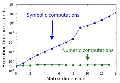
Symbolic computations becomes very slow with increase in matrix dimensions. For dimensions bigger than 15, there might even occur memory problems.

The preceding figure (Figure 15.3) illustrates the differences in CPU time between symbolically and numerically solving a linear system:

Figure 15.3: CPU time for numerically and symbolically solving a linear system.

Substitutions

Let us first consider a simple symbolic expression:

x, a = symbols('x a')
b = x + a

What happens if we set x = 0 ?  We observe that b did not change. What we did was that we changed the Python variable x. It now no longer refers to the symbol object but to the integer object 0. The symbol represented by the string 'x'  remains unaltered, and so does b.

Instead, altering an expression by replacing symbols by numbers, other symbols, or expressions is done by a special substitution method which can be seen in following code:

x, a = symbols('x a')
b = x + a
c = b.subs(x,0)   
d = c.subs(a,2*a)  
print(c, d)   # returns (a, 2a)

This method takes one or two arguments:

b.subs(x,0)
b.subs({x:0})  # a dictionary as argument

Dictionaries as arguments allow us to make several substitutions in one step:

b.subs({x:0, a:2*a})  # several substitutions in one

As items in dictionaries have no defined order - one never knows which would be the first - there is a need for...

Evaluating symbolic expressions

In the context of scientific computing, there is often the need of first making symbolic manipulations and then converting the symbolic result into a floating-point number .

The central tool for evaluating a symbolic expression is evalf. It converts symbolic expressions to floating-point numbers by using the following:

pi.evalf()   # returns 3.14159265358979

The data type of the resulting object is Float (note the capitalization), which is a SymPy data type that allows floating-point numbers with an arbitrary number of digits (arbitrary precision). The default precision corresponds to 15 digits, but it can be changed by giving evalf an extra positive integer argument specifying the desired precision in terms the numbers of digits,

pi.evalf(30)   # returns  3.14159265358979323846264338328

A consequence of working with arbitrary precision is that numbers can be arbitrary small, that is, the limits of the classical floating-point representation are broken; refer Floating...

Converting a symbolic expression into a numeric function

As we have seen the numerical evaluation of a symbolic expression is done in three steps, first we do some symbolic computations and then we substitute values by numbers and do an evaluation to a floating point number by evalf.

The reason for symbolic computations is often that one wants to make parameter studies. This requires that the parameter is modified within a given parameter range. This requires that an symbolic expression is eventually turned into a numeric function.

A study on the parameter dependency of polynomial coefficients

We demonstrate a symbolic/ numeric parameter study by an interpolation example to introduce the SymPy command lambdify. Let us consider the task to interpolate the data x = [0, t, 1] and y = [0, 1,-1]. Here, t is a free parameter, which we will vary over the interval [-0.4, 1.4]. The quadratic interpolation polynomial has coefficients depending on this parameter:

.

Using SymPy and the monomial approach...

Summary

In this chapter you were introduced in the world of symbolic computations and you got a glimpse of the power of SymPy. By guiding examples you learned how to set up symbolic expressions, how to work with symbolic matrices, and you saw how to make simplifications. Working with symbolic functions and transforming them into numerical evaluations built finally the link to scientific computing and floating point results. You experienced the strength of SymPy as you used its full integration into Python with its powerful constructs and legible syntax.

Consider this last chapter as an appetizer rather than a complete menu. We hope you became hungry for future fascinating programming challenges in scientific computing and mathematics.