7

A Primer on
Quaternions and Splines

Welcome to Chapter 7! In the previous chapter, we had a deeper view of the vector and matrix mathematical elements and data types. Both types are important building blocks of every 3D graphical application, as the internal storage and the calculation of virtual objects rely to a large extent on vertices and matrices.

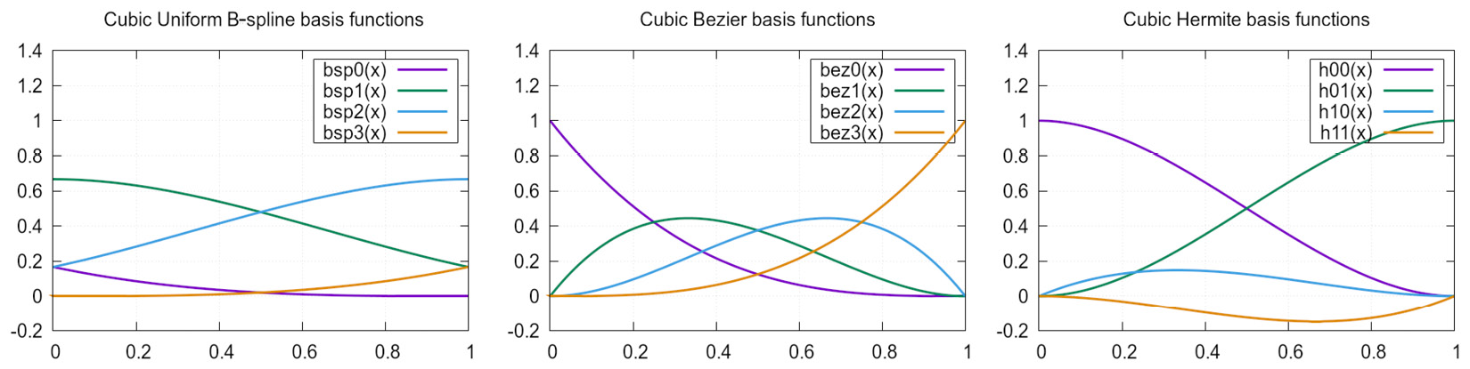
In this chapter, two other mathematical elements will be introduced: quaternions and splines, especially cubic Hermite splines. These two elements are heavily used in the glTF file format we use for the animated characters. The glTF file format will be explored in detail in Part 3 of the book, starting with Chapter 8.

By the end of the chapter, you should have a basic understanding of what quaternions and splines are, and how to work with them. You should also know about their advantages in character animations. Having a picture in your mind of the two elements and their transformations will help you master the rest of the...

Technical requirements

For this chapter, you will need the OpenGL and Vulkan renderer code from Chapter 6.

Working with game character animations requires a basic knowledge of quaternions, but you will find them in many other places in computer graphics applications too. So, let us look at what a quaternion is.

In this chapter, we will focus on the graphical output of example applications and show and describe only the parts of the code that do all the calculations. You can check out the full source in the subfolders of the chapter07 folder.

What are quaternions?

First, we need to check the mathematical elements that are required to describe and work with a quaternion. Without this, the quaternion is hard to understand.

Imaginary and complex numbers

If we try to solve this simple quadric equation, we are stuck if we are limited to the mathematical rules of the real numbers:

As the square of a number is always equal to or greater than zero and never negative, this equation has no result in the default mathematics world.

To be able to solve such equations, so-called imaginary numbers were introduced. The problem with equations like the one in the preceding formula is older than you may think: the basics of imaginary numbers have been known since the 15th century, and their usage was widely accepted in the 18th century.

To visualize the principle of imaginary numbers, a two-dimensional cartesian plane is used, as shown in Figure 7.1. The normal real numbers are on the horizontal x axis, while the imaginary...

Exploring vector rotation

Let us start with the most basic rotation we will have in the code, the natural-feeling rotation around the three axes in a three-dimensional cartesian space.

The Euler rotations

In the 18th century, the German mathematician Leonhard Euler (1707-1783) discovered the rule that a composition of two rotations in three-dimensional space is again a rotation, and these rotations differ only by the rotation axis.

We still use this rotation theorem today, to rotate objects around in virtual worlds. The final rotation of a three-dimensional object is a composition of rotations around the x, y, and z axis in three-dimensional cartesian space:

Figure 7.5: The three-dimensional cartesian space, plus the x, y, and z rotation axes

The rotations themselves are defined by the sine and cosine of the rotation angle:

Figure 7.6: Definition of the sine and the cosine of an angle

We are using the inverse of...

Using quaternions for smooth rotations

Spherical Linear Interpolation, or SLERP for short, uses mathematics to rotate from the position of one quaternion to the position of another quaternion. Figure 7.10 shows an example of SLERP. The red line is the path for the interpolation between the quaternions with orientations and .

Figure 7.10: Spherical Linear Interpolation between two quaternions

Doing the same transition with Euler angles works in one dimension. But for a full three-dimensional path between two quaternions, there is no simple mathematical solution to go from one combined rotation to another while maintaining a steady path in all the directions of the movement.

Note

Rotating from orientation and has a second solution: the other way around the circle, starting on and going “downward.” It is not guaranteed that Spherical Linear Interpolation will use the shortest path between two quaternions; this must be checked in the implementation...

A quick take on splines

In computer graphics, a spline is a curve, defined piecewise by polynomials. A polynomial for splines is a formula, where a single variable is used with different exponents and the results are summed up:

In the preceding formula, the first of the four base polynomials of a cubic Hermite spline is shown. Here, the t variable is used in a cubic and a squared version, and a real number is added to the polynomial.

Different spline variants use different polynomials to generate the resulting curved lines. The plots for the basic functions of the usually used spline variants – B-splines, Bezier, and Hermite splines – are drawn in Figure 7.12:

Figure 7.12: The basic functions for B-splines, Bezier, and Hermite splines

The construction of a spline can be done with numerical calculations, by solving all the polynomials for the given interpolation point between 0 and 1. Other splines can be created more easily by using...

Constructing a Hermite spline

A Hermit spline consists of four control points, split into two groups:

• A starting and ending vertex
• An incoming and an outgoing tangent

The right side of Figure 7.13 shows a Hermite spline. The two tangents start at the vertices: the incoming tangent begins at the start vertex, and the outgoing tangent starts at the end vertex.

Note

The incoming tangent of a Hermite spline points toward the direction of the spline path, and the outgoing tangent points away from the spline path.

The unequal directions of the two tangents may look a bit strange at first glimpse, as the Bezier spline on the left side of Figure 7.13 is completely inside the polygon created by the four control points. But this definition has a significant impact on the continuity of Hermite splines.

Spline continuity

If we want to join two splines, we must take care of the continuity of the spline path. Just setting the location of the starting vertex of the...

Summary

In this chapter, we introduced the two mathematical elements quaternion and spline, and the counterparts in GLM, ready to use in our code. After a brief discussion about the shortfalls of the usual three-dimensional rotation and the advantages of quaternions in character animations, we checked out splines and their usage in code.

All the steps from the first rotation to the quaternion/spline interpolation are accompanied by interactive code examples, ready to be tried out and to see the results of changing input values. These examples should have helped you to get a good insight into the possibilities of the two new data types.

In the next chapter, we start with the animation part of the book. The first step will be the exploration of the file format, the components inside it, what we need from the data, and which parts can be left out.

Practical sessions

Here are some ideas if you want to get a deeper insight into quaternions and splines:

• Join multiple Hermite splines in the 06_opengl_spline_quat and/or 12_vulkan_spline_quat examples to create a bigger spline and interpolate the moving box from the last example code along all of the splines. To continuously join two Hermite splines, the end vertex of the first spline needs to be the starting vertex of the second spline, and the output tangent of the first spline needs to be the input tangent of the second spline. Switching between the different splines may be a bit tricky though.
• Enhanced difficulty level: Assign different lengths of the overall interpolation range to the splines. This leads to different movement speeds of the box on the splines. One spline may take, say, 80% of the interpolation range, resulting in a slow-moving box along the path, while the others share the remaining 20%, and the box will move much faster along the path.
• Add some...

Additional resources

• The quaternion explanation from 3D Game Engine Programming: https://www.3dgep.com/understanding-quaternions/
• Quaternions in the OpenGL tutorial: http://www.opengl-tutorial.org/intermediate-tutorials/tutorial-17-quaternions/
• An interactive demo of a 2D cubic Hermite interpolation: http://demofox.org/cubichermite2d.html