

Classification is another kind of supervised machine learning. In this chapter, before getting into the details of building a classification model using ML Studio, you will start with gaining the basic knowledge about a classification algorithm and how a model is evaluated. Then, you will build models with different datasets using different algorithms.

Consider you are given the following hypothetical dataset containing data of patients: the size of the tumor in their body, their age, and a class that justifies whether they are affected by cancer or not, 1 being positive (affected by cancer) and 0 being negative (not affected by cancer):
|
Age |
Tumor size |
Class |
|---|---|---|
|
22 |
135 |
0 |
|
37 |
121 |
0 |
|
18 |
156 |
1 |
|
55 |
162 |
1 |
|
67 |
107 |
0 |
|
73 |
157 |
1 |
|
36 |
123 |
0 |
|
42 |
189 |
1 |
|
29 |
148 |
0 |
Here, the patients are classified as cancer-affected or not. A new patient comes in at the age 17 and is diagnosed of having a tumor the of size 149. Now, you need to predict the classification of this new patient based on the previous data. That's classification for you as you need to predict the class of the dependent variable; here it is 0 or 1—you may also think of it as true or false.
For a regression problem, you predict a number, for example, the housing price or a numerical value. In a classification problem, you predict a categorical value...
As with regression problems, which you saw in the previous chapter, with classification problems, you can start with an algorithm and train it with data. You can then score ideally with the test data and evaluate the performance of the model.
Navigate to the Train | Score | Evaluate option on the screen.
The Train, Score, and Evaluate modules are the same as you used for regression. The Train module requires the name of the target (class) variable. The Evaluate module generates evaluation metrics for classification.
If you want to tune parameters of an algorithm by parameter sweeping, you can use the same Sweep Parameters module.
The Pima Indians Diabetes Binary Classification dataset module is present as a sample dataset in ML Studio. It contains all of the data of female patients of the same age belonging to Pima Indian heritage. The data includes medical data, such as glucose and insulin levels, as well as lifestyle factors of the patients. The columns in the dataset are as follows:
Number of times pregnant
Plasma glucose concentration of 2 hours in an oral glucose tolerance test
Diastolic blood pressure (mm Hg)
Triceps skin fold thickness (mm)
2-hour serum insulin (mu U/ml)
Body mass index (weight in kg/(height in m)^2)
Diabetes pedigree function
Age (years)
Class variable (0 or 1)
The last column is the target variable or class variable that takes the value 0 or 1, where 1 is positive or affected by diabetes and 0 means that the patient is not affected.
You have to build models that could predict whether a patient has diabetes or tests positive or not.
ML Studio comes with three decision-tree-based algorithms for two-class classification: the Two-Class Decision Forest, Two-Class Boosted Decision Tree, and Two-Class Decision Jungle modules. These are known as ensemble models where more than one decision trees are assembled to obtain better predictive performance. Though all the three are based on decision trees, their underlying algorithms differ.
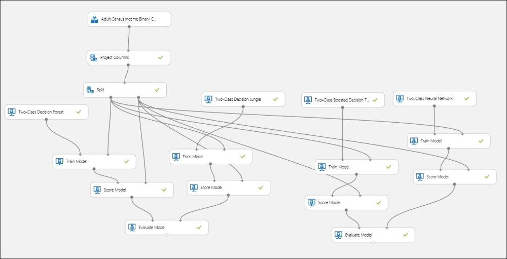
We will first build a model with the Two-Class Decision Forest module and then compare it with the Two-Class Boosted Decision Tree module for the Adult Census Income Binary Classification dataset module, which is one of the sample datasets available in ML Studio. The dataset is a subset of the 1994 US census database and contains the demographic information of working adults over the 16 years age limit. Each instance or example in the dataset has a label or class variable that states whether a person earns 50K a year or not.
You have already tried two algorithms for the Adult Census Income Binary Classification dataset module. Now, try another two modules to choose the best one for your final model: the Two-Class Boosted Decision Tree and the Two-Class Neural Network modules. Try out different parameters; use the Sweep Parameters module to optimize the parameters for the algorithms. The following screenshot is just for your reference—your experiment might differ. You may also try this with other available algorithms, for example, the Two-Class Averaged Perceptron or the Two-Class Logistic Regression modules to find the best model. Let's take a look at the following screenshot:
The classification you have seen and experienced so far is a two-class classification where the target variable can be of two classes. In multiclass classification, you classify in more than two classes, for example continuing on our hypothetical tumor problem, for a given tumor size and age of a patient, you might predict one of these three classes as the possibility of a patient being affected with cancer: High, Medium, and Low. In theory, a target variable can have any number of classes.
ML Studio lets you evaluate your model with an accuracy that is calculated as a ratio of the number of correct predictions versus the incorrect ones. Consider the following table:
|
Age |
Tumor size |
Actual class |
Predicted class |
|---|---|---|---|
|
32 |
135 |
Low |
Medium |
|
47 |
121 |
Medium |
Medium |
|
28 |
156 |
Medium |
High |
|
45 |
162 |
High |
High |
|
77 |
107 |
Medium |
Medium |
The following can be the evaluation metrics where in the columns, the text is marked in bold...
The Iris dataset is one of the classic and simple datasets. It contains the observations about the Iris plant. Each instance has four features: the sepal length, sepal width, petal length, and petal width. All the measurements are in centimeters. The dataset contains three classes for the target variable, where each class refers to a type of Iris plant: Iris Setosa, Iris Versicolour, and Iris Virginica.
You can find more information on this dataset at http://archive.ics.uci.edu/ml/datasets/Iris.
As this dataset is not present as a sample dataset in ML Studio, you need to import it to ML Studio using a reader module before building any model on it. Note that the Iris dataset present in the Saved Dataset section is the subset of the original dataset and is only present for two classes.
The Wine dataset is another classic and simple dataset hosted in the UCI machine learning repository. It contains chemical analysis of the content of wines grown in the same region in Italy, but derived from three different cultivars. It is used to determine models for classification problems by predicting the source (cultivar) of wine as class or target variable. The dataset has the following 13 features (dependent variables), which are all numeric:
Alcohol
Malic acid
Ash
Alcalinity of ash
Magnesium
Total phenols
Flavanoids
Nonflavanoid phenols
Proanthocyanins
Color intensity
Hue
OD280/OD315 of diluted wines
Proline
The examples or instances are classified into three classes: 1, 2 and 3.
You can find more about the dataset at http://archive.ics.uci.edu/ml/datasets/Wine.
You started the chapter with understanding predictive analysis with classification and explored the concepts of training, testing, and validating a classification model. You then proceeded to carry on building experiments with different two-class and multiclass classification models, such as logistic regression, decision forest, neural network, and boosted decision trees inside ML Studio. You learned how to score and evaluate a model after training. You also learned how to optimize different parameters for a learning algorithm by the module, Sweep Parameters.
After exploring the two-class classification, you understood multiclass classification and learnt how to evaluate a model for the same. You then built a couple of models for multiclass classification using different available algorithms.
In the next chapter, you will explore the process of building a model using clustering, an unsupervised learning algorithm.
The rest of the chapter is locked
You have been reading a chapter from
Microsoft Azure Machine LearningPublished in: Jun 2015Publisher: ISBN-13: 9781784390792
Register for a free Packt account to unlock a world of extra content!
A free Packt account unlocks extra newsletters, articles, discounted offers, and much more. Start advancing your knowledge today.
undefined
Unlock this book and the full library FREE for 7 days
Get unlimited access to 7000+ expert-authored eBooks and videos courses covering every tech area you can think of
Renews at $15.99/month. Cancel anytime