Special Purpose Plots

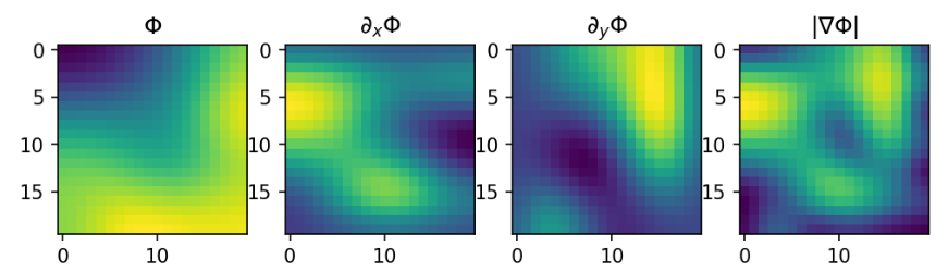
We have so far learned how to add lines, boxes, texts, different kinds of shapes, as well as arrows in descriptions with annotation. Special purpose plots defines how to draw on plots to provide the viewer with visual guides that point them toward the important features of data and a few special purpose kinds of plots for either plotting non-Cartesian data or very specific kinds of datasets.

In this chapter, we will learn about the following topics:

• How to make non-Cartesian axes and plots
• How to plot vector fields
• How to show statistical information with box and violin plots
• How to display ordinal and tabular data

Non-Cartesian plots

We will begin by importing all the necessary packages, as follows:

import numpy as np
import matplotlib as mpl
import matplotlib.pyplot as plt
%matplotlib inline
# Set up figure size and DPI for screen demo
plt.rcParams['figure.figsize'] = (6,4)
plt.rcParams['figure.dpi'] = 150

Creating polar axes

First, we will bring up a simple plot with the following code:

nums = np.arange(0,10,0.1)
plt.plot(nums, nums/10.)
plt.plot(nums, np.sin(nums))
plt.plot(nums, np.cos(nums))

The preceding code will give the following output:

The preceding output shows a sine and cosine plot, with a linear plot alongside it. We will take a look at the cosine and sine plot, but not as a function of its linear length....

Plotting vector fields

First, though, we will generate a standard Gaussian random field so that we have a nice gradient:

# Generate a vector field with a gradient
from scipy.ndimage.filters import gaussian_filter
x = np.arange(0,10,0.5)
y = np.arange(0,10,0.5)
phi = gaussian_filter(np.random.uniform(size=(20,20)), sigma=5)
plt.subplot(141)
plt.imshow(phi, interpolation='none')
plt.title(r'$\Phi$')
plt.subplot(142)
plt.imshow(np.gradient(phi)[0], interpolation='none')
plt.title(r'$\partial_x\Phi$')
plt.subplot(143)
plt.title(r'$\partial_y\Phi$')
plt.imshow(np.gradient(phi)[1], interpolation='none')
plt.subplot(144)
plt.title(r'$\|\nabla \Phi\|$')
plt.imshow(np.linalg.norm(np.gradient(phi), axis=0), interpolation='none')
plt.gcf().set_size_inches(8,4)

Following is the output of the preceding code:

Let's take look...

Statistics with boxes and violins

This section describes how to make box plots and outliers within the data and how to customize the appearance of plots.

Making box plots to show the interquartile ranges and the outliers

We will begin by importing the data. Start by generating normal Gaussian distributions with a couple of different properties, as follows:

# Generate some Normal distributions with different properties
rands1 = np.random.normal(size=500)
rands2 = np.random.normal(scale=2, size=500)
rands3 = np.random.normal(loc=1, scale=0.5, size=500)
gaussians = (rands1, rands2, rands3)

1. Make some box plots out of this data. Hence, by making a box plot of Gaussians, we can comment to suppress the output. Here, we can see that...

Visualizing ordinal and tabular data

In this section, we will talk about tabular and ordinal data, where we don't have an x axis and y axis. We're going to take a look at the following topics:

• Pie charts
• Tables
• How to customize the appearance of plots

Pie charts

Let's take a look at the fractions of gases that exist in our atmosphere. The following content shows the code and output for Nitrogen, which is 78 percent of our atmosphere, Oxygen, which is 21 percent, and Argon, which is 1 percent. Now, naturally, Nitrogen, Oxygen, and Argon are not exactly numerical values. Hence, we cannot really plot these things against each other in the standard way. This is where we can use a pie chart as a best practice to...

Summary

In this chapter, we learned how to plot on non-Cartesian axes and how to plot high-dimensional vector field data. We also studied how to plot different kinds of statistical distributions with box and violin plots. Finally, we learned how to display small numbers of ordinal and tabular data with pie charts and tables.

In the next chapter, we will look at how to plot 3D and geospatial data.