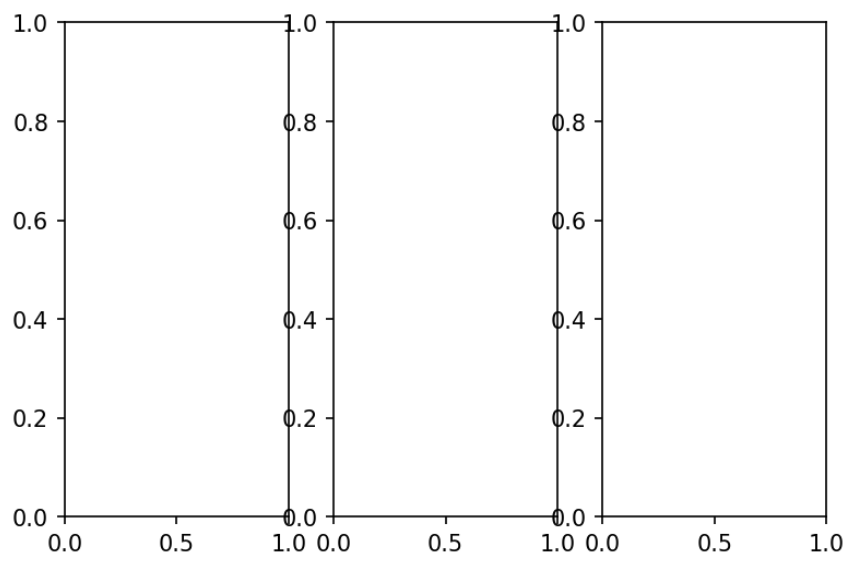
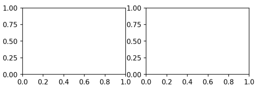
We will begin by looking at a subplot with one set of rows and three columns, as shown here:
# Standard Subplot
plt.subplot(131)
plt.subplot(132)
plt.subplot(133)
The following is the output of the preceding input:
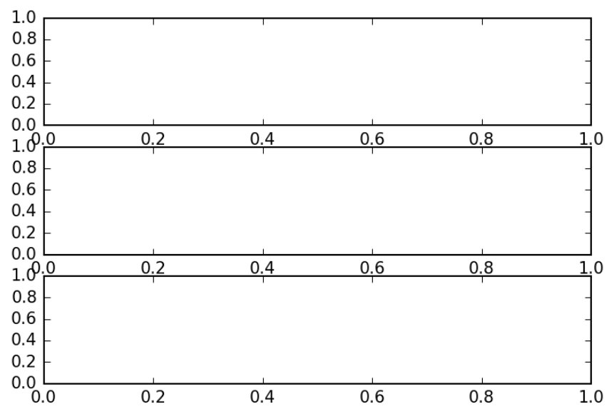
Now, by default, it will provide three plots side by side of equal size, but if we want them on top of each other instead, we will choose three rows and one column:
# Standard Subplot
plt.subplot(311)
plt.subplot(312)
plt.subplot(313)
We will get the following output:
But what if these plots aren't necessarily supposed to show three identical ranges? In that case, we have the subplot2grid method:
# subplot2grid
plt.subplot2grid((2,2), (0,0))
plt.subplot2grid((2,2), (1,0))
plt.subplot2grid((2,2), (0,1))
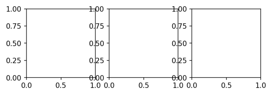
We will begin by making the same vertical plot as shown previously. Now, specify one row and three columns and in the second tuple, select the rows, because there's only one and three columns. Next, we will see that there's a grid with two rows and three columns. We will place everything in the first column within the first row and simply specify a column:
# subplot2grid
plt.subplot2grid((2,3), (0,0))
plt.subplot2grid((2,3), (0,1))
plt.subplot2grid((2,3), (0,2))
The output will be as follows:
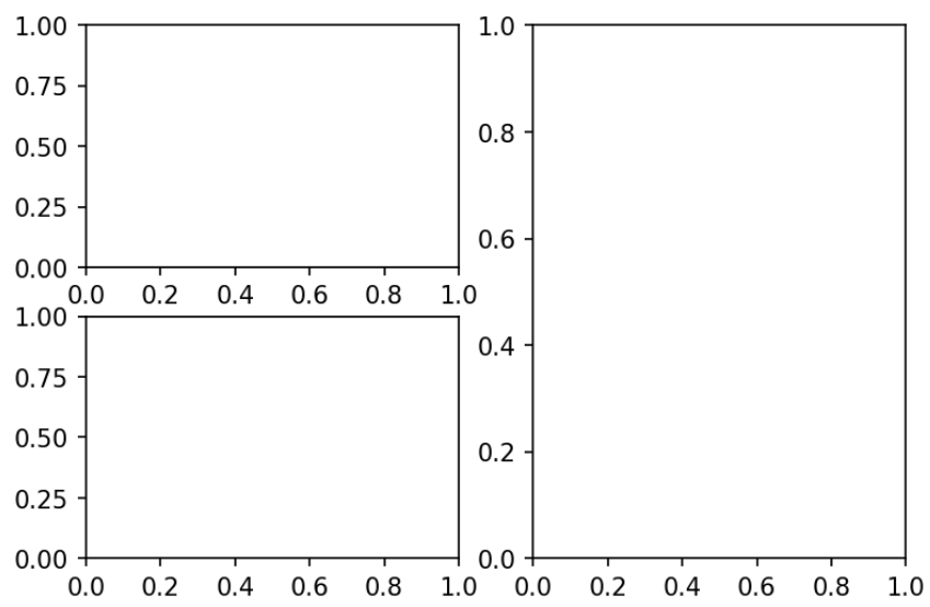
Now, to get this in a 2 x 3 grid, we need to have two plots underneath a third one; well in that case, what we want is a 2 x 2 grid, so one plot is going to be twice as wide and then two plots beneath, as shown here:
# Adjusting GridSpec attributes: w/h space
gs = mpl.gridspec.GridSpec(2,2)
plt.subplot(gs[0,0])
plt.subplot(gs[1,0])
plt.subplot(gs[1,1])
We will get the following output:
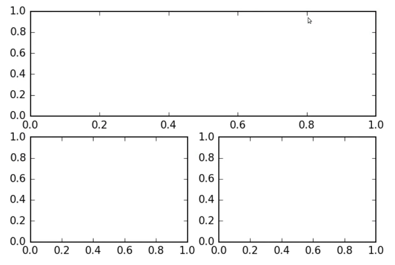
We have the positions right, but this has not actually made the plots bigger. To do that, we will have to pass an argument to the first one, plt.subplot2grid, called colspan=2, and using colspan, we say that this plot should span as shown in the following code:
# subplot2grid
plt.subplot2grid((2,2), (0,0), colspan=2)
plt.subplot2grid((2,2), (1,0))
plt.subplot2grid((2,2), (0,1))
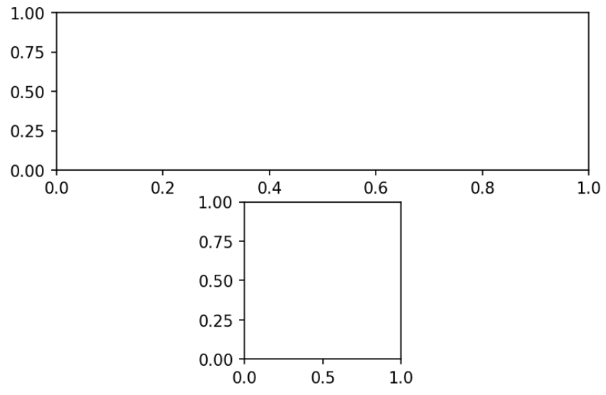
We will get the following output::
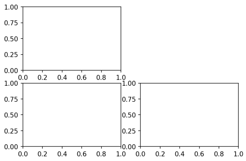
There is also another option as well for doing similar things, but in the vertical direction with row span. Therefore, we can perform the following action:
# subplot2grid
plt.subplot2grid((2,2), (0,0))
plt.subplot2grid((2,2), (1,0))
plt.subplot2grid((2,2), (0,1), rowspan=2)
From the preceding code, we will get the following output:
We can do the same thing using a GridSpec object and in fact we can customize this a little more explicitly. After creating a GridSpec object, iterate it through the indices of that GridSpec to say where it will get placed. These indices are just like any two-dimensional NumPy array. So, for example, we can perform the following:
# Explicit GridSpec
gs = mpl.gridspec.GridSpec(2,2)
plt.subplot(gs[0,0])
plt.subplot(gs[0,1])
The following is the output of the preceding code:
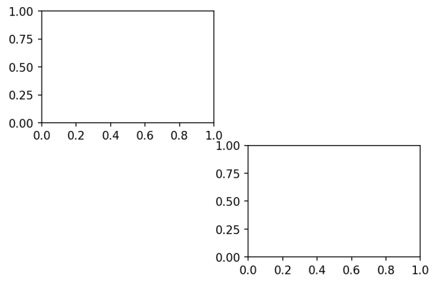
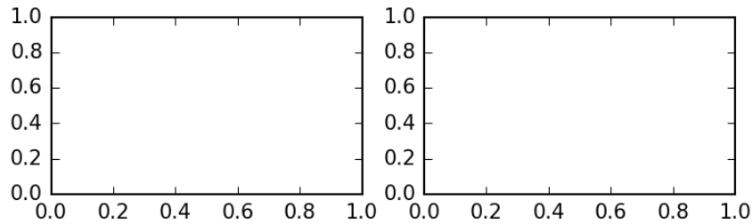
By including a diagonal pair of plots, we get the following:
# Explicit GridSpec
gs = mpl.gridspec.GridSpec(2,2)
plt.subplot(gs[0,0])
plt.subplot(gs[1,1])
We will get the following output:
We can also make those plots span things using the range syntax that NumPy provides for us:
# Explicit GridSpec
gs = mpl.gridspec.GridSpec(2,2)
plt.subplot(gs[0,:])
plt.subplot(gs[1,1])
The preceding code gives the following output:
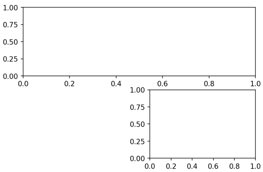
If, for example, we made this have three columns, we would get the following:
# Explicit GridSpec
gs = mpl.gridspec.GridSpec(2,3)
plt.subplot(gs[0,:])
plt.subplot(gs[1,1])
We will get the following output:
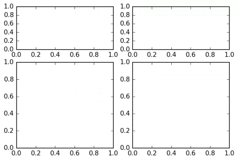
This shows that we can really dive into providing whatever kind of grid-like layout we want with plots of different sizes and shapes. You can also customize the amount of space between these plots. For example, look at the following grid:
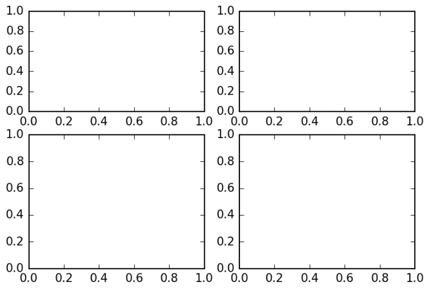
We can adjust the amount of space between the grids using wspace for space between the plots:
# Adjusting GridSpec attributes: w/h space
gs = mpl.gridspec.GridSpec(2,2, wspace=0.5)
plt.subplot(gs[0,0])
plt.subplot(gs[0,1])
plt.subplot(gs[1,0])
plt.subplot(gs[1,1])
The preceding code gives the following output:
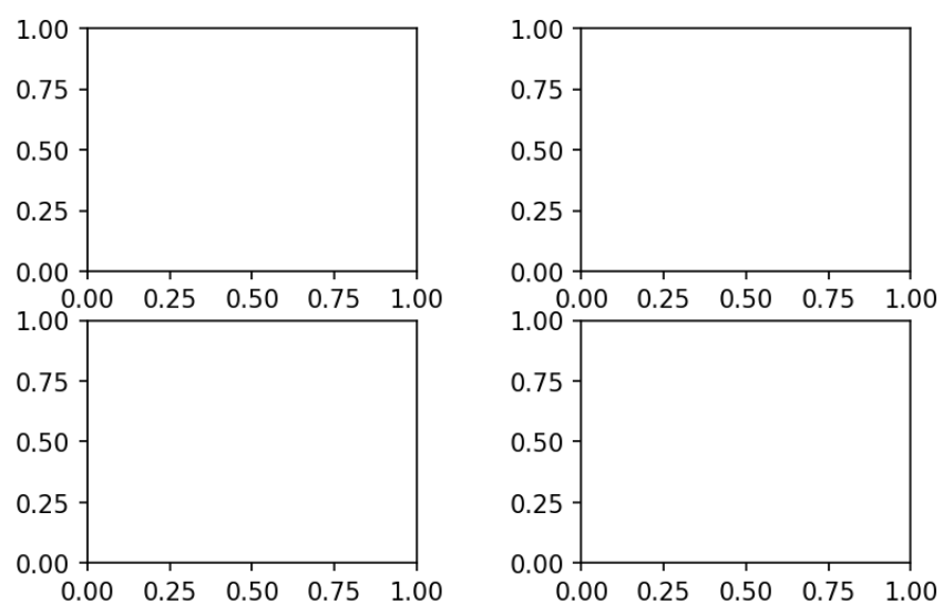
We can also adjust the amount of space between the grids using hspace for space between the plots:
# Adjusting GridSpec attributes: w/h space
gs = mpl.gridspec.GridSpec(2,2, hspace=0.5)
plt.subplot(gs[0,0])
plt.subplot(gs[0,1])
plt.subplot(gs[1,0])
plt.subplot(gs[1,1])
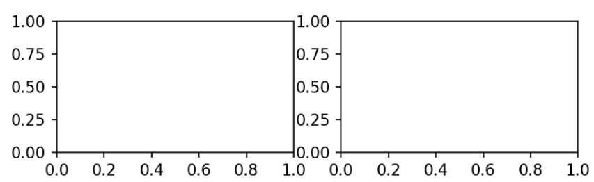
The ratios of the sizes can also be changed between the plots. So, say, for example, that we want our top row to be very tall and thin; we can specify a width and height ratio. If we pass width_ratios, we can decide how big each of these columns will appear relative to one another in terms of their width:
# Adjusting GridSpec attributes: width/height ratio
gs = mpl.gridspec.GridSpec(2,2, width_ratio=(1,2))
plt.subplot(gs[0,0])
plt.subplot(gs[0,1])
plt.subplot(gs[1,0])
plt.subplot(gs[1,1])
It sets the width of the second column to be twice the width of the first column:
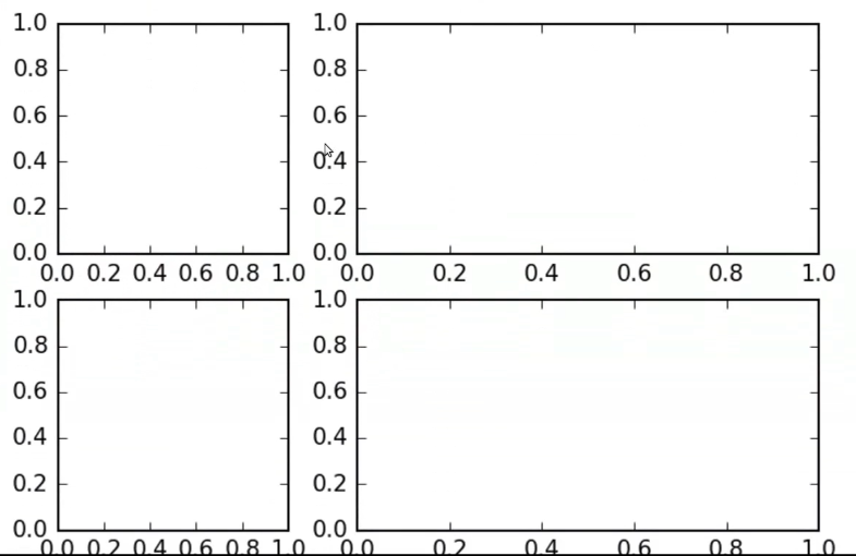
When changing this to (2, 2), they will be equal, so it will literally just take a ratio of these numbers; you can pass whatever pair of ratios you want:
# Adjusting GridSpec attributes: width/height ratio
gs = mpl.gridspec.GridSpec(2,2, width_ratio=(2,2))
plt.subplot(gs[0,0])
plt.subplot(gs[0,1])
plt.subplot(gs[1,0])
plt.subplot(gs[1,1])
We will get the following output:
By changing the heights, we get the second set of plots—twice the height of the first one, as shown here:
# Adjusting GridSpec attributes: width/height ratio
gs = mpl.gridspec.GridSpec(2,2, height_ratio=(1,2))
plt.subplot(gs[0,0])
plt.subplot(gs[0,1])
plt.subplot(gs[1,0])
plt.subplot(gs[1,1])
We will see the following output:
These cannot only be integers—they can be floating-point numbers as well, as shown here:
# Adjusting GridSpec attributes: width/height ratio
gs = mpl.gridspec.GridSpec(2,2, height_ratios=(1.5,2))
plt.subplot(gs[0,0])
plt.subplot(gs[0,1])
plt.subplot(gs[1,0])
plt.subplot(gs[1,1])
By executing the preceding code, we will get the following output:
Hence, this is a quick and convenient way of setting up multi-panel plots that put the focus on the kinds of plots that we want to dominate. So, if you have a situation where, for example, you have a complex dataset where one piece of that visualization is the most important one but you have many supplemental plots that you want to show alongside it, using the subplot two grid and the grid spec object can be a nice way of building up those layouts.