Reader small image

You're reading from  Learning Quantitative Finance with R

Product typeBook
Published inMar 2017
Reading LevelIntermediate
PublisherPackt
ISBN-139781786462411
Edition1st Edition
Languages
Right arrow
Authors (2):
Dr. Param Jeet
Dr. Param Jeet
author image
Dr. Param Jeet

Dr. Param Jeet is a Ph.D. in mathematics from one of India's leading technological institute in Madras (IITM), India. Dr. Param Jeet has a couple of mathematical research papers published in various international journals. Dr. Param Jeet has been into the analytics industry for the last few years and has worked with various leading multinational companies as well as consulted few of companies as a data scientist.
Read more about Dr. Param Jeet

PRASHANT VATS
PRASHANT VATS
author image
PRASHANT VATS

Prashant Vats is a masters in mathematics from one of India's leading technological institute, IIT Mumbai. Prashant has been into analytics industry for more than 10 years and has worked with various leading multinational companies as well as consulted few of companies as data scientist across several domain.
Read more about PRASHANT VATS

View More author details
Right arrow

AR


AR stands for autoregressive model. Its basic concept is that future values depend on past values and they are estimated using a weighted average of the past values. The order of the AR model can be estimated by plotting the autocorrelation function and partial autocorrelation function of the series. In time series autocorrelation function measures correlation between series and it's lagged values. Whereas partial autocorrelation function measures correlation of a time series with its own lagged values, controlling for the values of the time series at all shorter lags. So first let us plot the acf and pcf of the series. Let us first plot the acf plot by executing the following code:

> PriceData<-ts(StockData$Adj.Close, frequency = 5) 
> acf(PriceData, lag.max = 10) 

This generates the autocorrelation plot as displayed here:

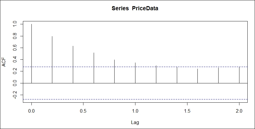
Figure 4.5: acf plot of price

Now let us plot pacf by executing the following code:

> pacf(PriceData, lag.max = 10) 

This generates the partial autocorrelation...

lock icon
The rest of the page is locked
Previous PageNext Page
You have been reading a chapter from
Learning Quantitative Finance with R
Published in: Mar 2017Publisher: PacktISBN-13: 9781786462411

Authors (2)

author image
Dr. Param Jeet

Dr. Param Jeet is a Ph.D. in mathematics from one of India's leading technological institute in Madras (IITM), India. Dr. Param Jeet has a couple of mathematical research papers published in various international journals. Dr. Param Jeet has been into the analytics industry for the last few years and has worked with various leading multinational companies as well as consulted few of companies as a data scientist.
Read more about Dr. Param Jeet

author image
PRASHANT VATS

Prashant Vats is a masters in mathematics from one of India's leading technological institute, IIT Mumbai. Prashant has been into analytics industry for more than 10 years and has worked with various leading multinational companies as well as consulted few of companies as data scientist across several domain.
Read more about PRASHANT VATS