Reader small image

You're reading from  Learning Quantitative Finance with R

Product typeBook
Published inMar 2017
Reading LevelIntermediate
PublisherPackt
ISBN-139781786462411
Edition1st Edition
Languages
Right arrow
Authors (2):
Dr. Param Jeet
Dr. Param Jeet
author image
Dr. Param Jeet

Dr. Param Jeet is a Ph.D. in mathematics from one of India's leading technological institute in Madras (IITM), India. Dr. Param Jeet has a couple of mathematical research papers published in various international journals. Dr. Param Jeet has been into the analytics industry for the last few years and has worked with various leading multinational companies as well as consulted few of companies as a data scientist.
Read more about Dr. Param Jeet

PRASHANT VATS
PRASHANT VATS
author image
PRASHANT VATS

Prashant Vats is a masters in mathematics from one of India's leading technological institute, IIT Mumbai. Prashant has been into analytics industry for more than 10 years and has worked with various leading multinational companies as well as consulted few of companies as data scientist across several domain.
Read more about PRASHANT VATS

View More author details
Right arrow

Chapter 4.  Time Series Modeling

Time series forecasting analysis is one of the most important components of quantitative finance. R software gives a lot of time series and forecasting packages to support time series analysis. There are sufficient packages in R to convert the equally spaced and unequally spaced series in time series. Also, there are sufficient packages in R to build forecasting models such as autoregressive integrated moving average and generalized autoregressive conditional heteroscedasticity. In this chapter, we are going to give brief flavors of converting any series into time series and forecasting models.

In this chapter, we are going to cover the following topics:

  • General time series

  • Converting data to time series

  • zoo

  • xts

  • Linear filters

  • AR

  • MA

  • ARIMA

  • GARCH

  • EGARCH

  • VGARCH

  • Dynamic conditional correlation

General time series


A time series is the sequence of data usually collected at regular intervals. There are a lot of domains where information is stored in time series form and needs to be analyzed for future planning.

For example, in the financial domain, we have the daily/monthly data available for unemployment, GDP, daily exchange rates, share prices, and so on. So all the investors or the people working in financial institutions need to plan their future strategy and so they want to analyze the time series data. Thus time series play a crucial role in the financial domain.

Time series data is very unpredictable in nature and to understand the data we need to decompose the time series data into various components, as given here:

  • Trend: This is a pattern of long-term movements in the mean of time series data. The trend may be linear or nonlinear and keeps changing across time. There is no sure process to identify the exact trend but if it is behaving monotonously then it is possible to estimate...

Converting data to time series


A time series is a sequence of data points where each data point is associated with a particular time.

For example, the adjusted close of a stock is the closing price of a stock on a particular day. The time series data is stored in an R object called a time series object and it is created by using the function ts() in R.

The basic syntax of ts is given here:

ts(data, start, end, frequency) 

Here:

  • data: It is a vector or matrix containing the data values

  • start: It is the starting point or time of first observation

  • end: It is the time point of last observation

  • frequency: It is the number of data points per unit time

Let us consider a vector which is given by the following code:

> StockPrice<
-c(23.5,23.75,24.1,25.8,27.6,27,27.5,27.75,26,28,27,25.5) 
> StockPrice 

Now convert it into a time series object, which can be done with the following code:

> StockPricets<- ts(StockPrice,start = c(2016,1),frequency = 12)   
> StockPricets  

The output is as...

zoo


The ts object has its limitations in representing the time series. It is used for representing equally spaced data. It cannot be used to represent the daily level stock prices as stock prices are equally spaced between Monday to Friday, but it is not the same case for Friday to Monday and in case there is market holidays on weekdays. This type of unequally spaced data cannot be represented by a ts object.

zoo is flexible and fully equipped to handle unequally spaced data, equally spaced data, and numerically indexed data.

Let us first install and load the zoo library. This can be done by executing the following code:

> install.packages("zoo") 
> library(zoo) 

Now we will discuss how to represent different time series scenarios using zoo.

Please note we will be using a common dataset for all the examples.

Constructing a zoo object

In order to create a zoo object, an ordered time index and data are required. So we are going to construct a zoo object.

Let us first import a few rows of our...

xts


xts is an extensible time series object which carries all the features of a zoo object. It consists of a matrix and index which has to be time-based. There are two ways of constructing xts objects: one is by calling as.xts and another is constructing the xts object from scratch.

Construction of an xts object using as.xts

Let us read a few lines of our sample data through zoo and construct the xts object by executing the following code:

> StockData <- read.zoo("DataChap4.csv",header = TRUE, sep = ",",format="%m/%d/%Y",nrows=3) 
> matrix_xts <- as.xts(StockData,dateFormat='POSIXct') 
> matrix_xts 

This gives the following output:

Volume

Adj.Close

Return

12/12/2016

615800

192.43

0.13

12/13/2016

6816100

198.15

2.97

12/14/2016

4144600

198.69

0.27

The composition of the xts object can be given by the following code:

> str(matrix_xts) 

This generates the following output:

An xts object on 2016-12-12/2016-12-14 contains the following:

  Data: num [1:3, 1:3]...

Linear filters


The first step in time series analysis is to decompose the time series in trend, seasonality, and so on.

One of the methods of extracting trend from the time series is linear filters.

One of the basic examples of linear filters is moving average with equal weights.

Examples of linear filters are weekly average, monthly average, and so on.

The function used for finding filters is given as follows:

Filter(x,filter)

Here, x is the time series data and filter is the coefficients needed to be given to find the moving average.

Now let us convert the Adj.Close of our StockData in time series and find the weekly and monthly moving average and plot it. This can be done by executing the following code:

> StockData <- read.zoo("DataChap4.csv",header = TRUE, sep = ",",format="%m/%d/%Y") 
>PriceData<-ts(StockData$Adj.Close, frequency = 5)
> plot(PriceData,type="l")
> WeeklyMAPrice <- filter(PriceData,filter=rep(1/5,5))
> monthlyMAPrice <- filter(PriceData,filter=rep...

AR


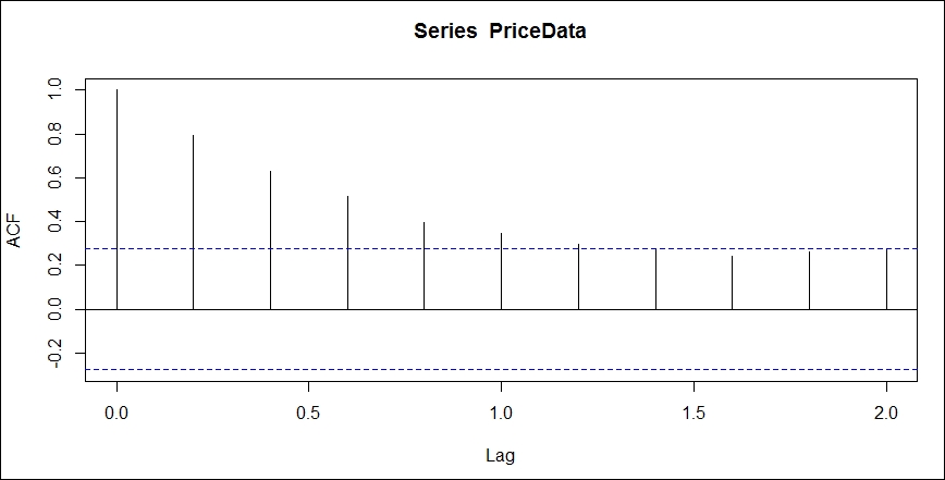
AR stands for autoregressive model. Its basic concept is that future values depend on past values and they are estimated using a weighted average of the past values. The order of the AR model can be estimated by plotting the autocorrelation function and partial autocorrelation function of the series. In time series autocorrelation function measures correlation between series and it's lagged values. Whereas partial autocorrelation function measures correlation of a time series with its own lagged values, controlling for the values of the time series at all shorter lags. So first let us plot the acf and pcf of the series. Let us first plot the acf plot by executing the following code:

> PriceData<-ts(StockData$Adj.Close, frequency = 5) 
> acf(PriceData, lag.max = 10) 

This generates the autocorrelation plot as displayed here:

Figure 4.5: acf plot of price

Now let us plot pacf by executing the following code:

> pacf(PriceData, lag.max = 10) 

This generates the partial autocorrelation...

MA


MA stands for moving average and in MA modeling we do not take into account the past values of the actual series. We consider the moving average of the past few forecast errors in this process. For identifying the orders of MA, we also need to plot acf and pacf. So let us plot the acf and pacf of the volume of StockData to evaluate the order of MA. acf can be plotted by executing the following code:

> VolumeData<-ts(StockData$Volume, frequency = 5) 
> acf(VolumeData, lag.max = 10) 

This gives the following acf plot:

Figure 4.7: acf plot of volume

Let us plot the pacf plot of volume by executing the following code:

> pacf(VolumeData, lag.max = 10) 

This gives the following plot:

Figure 4.8: pacf plot of volume

After evaluating the preceding plots, the acf cuts sharply after lag1 so the order of MA is 1.

ARIMA


ARIMA stands for autoregressive integrated moving average models. Generally, it is defined by the equation ARIMA(p, d, q).

Here,

  • p is the order of the autoregressive model

  • d is the order required for making the series stationary

  • q is the order of moving average

The very first step in ARIMA is to plot the series, as we need a stationary series for forecasting.

So let us first plot the graph of the series by executing the following code:

> PriceData<-ts(StockData$Adj.Close, frequency = 5) 
> plot(PriceData) 

This generates the following plot:

Figure 4.9: Plot of price data

Clearly, upon inspection, the series seems to be nonstationary, so we need to make it stationary by differencing. This can be done by executing the following code:

> PriceDiff <- diff(PriceData, differences=1) 
> plot(PriceDiff) 

This generates the following plot for the differenced series:

Figure 4.10: Plot of differenced price data

This is a stationary series, as the means and variance seem to be constant...

GARCH


GARCH stands for generalized autoregressive conditional heteroscedasticity. One of the assumptions in OLS estimation is that variance of error should be constant. However, in financial time series data, some periods are comparatively more volatile, which contributes to rise in strengths of the residuals, and also these spikes are not randomly placed due to the autocorrelation effect, also known as volatility clustering, that is, periods of high volatility tend to group together. This is where GARCH is used to forecast volatility measures, which can be used to forecast residuals in the model. We are not going to go into great depth but we will show how GARCH is executed in R.

There are various packages available in R for GARCH modeling. We will be using the rugarch package.

Let us first install and load the rugarch package, which can be done by executing the following code:

>install.packages("rugarch") 
>Library(rugarch) 
 >snp <- read.zoo("DataChap4SP500.csv",header = TRUE...

EGARCH


EGARCH stands for exponential GARCH. EGARCH is an improved form of GARCH and models some of the market scenarios better.

For example, negative shocks (events, news, and so on) tend to impact volatility more than positive shocks.

This model differs from the traditional GARCH in structure due to the log of variance.

Let us take an example to show how to execute EGARCH in R. First define spec for EGARCH and estimate the coefficients, which can be done by executing the following code on the snp data:

> snp <- read.zoo("DataChap4SP500.csv",header = TRUE, sep = ",",format="%m/%d/%Y") 
> egarchsnp.spec = ugarchspec(variance.model=list(model="eGARCH",garchOrder=c(1,1)), 
+                        mean.model=list(armaOrder=c(0,0))) 
> egarchsnp.fit = ugarchfit(egarchsnp.spec, snp$Return) 
> egarchsnp.fit 
> coef(egarchsnp.fit) 

This gives the coefficients as follows:

Figure 4.19: Parameter estimates of EGARCH

Now let us try to forecast, which can be done by executing the following...

VGARCH


VGARCH stands for vector GARCH or multivariate GARCH. In the financial domain, the assumption is that financial volatilities move together over time across assets and markets. Acknowledging this aspect through a multivariate modeling framework leads to a better model separate univariate model. It helps in making better decision tools in various areas, such as asset pricing, portfolio selection, option pricing, and hedging and risk management. There are multiple options in R for building in multivariate mode.

Let us consider an example of multivariate GARCH in R for the last year of data from the S&P500 and DJI index:

>install.packages("rmgarch")
>install.packages("PerformanceAnalytics")
>library(rmgarch)
>library(PerformanceAnalytics)
>snpdji <- read.zoo("DataChap4SPDJIRet.csv",header = TRUE, sep = ",",format="%m/%d/%Y")
>garch_spec = ugarchspec(mean.model = list(armaOrder = c(2,1)),variance.model = list(garchOrder = c(1,1), model = "sGARCH"), distribution.model...

Dynamic conditional correlation


Multivariate GARCH models, which are linear in squares and cross products of the data, are generally used to estimate the correlations changing with time. Now this can be estimated using dynamic conditional correlation (DCC), which is a combination of a univariate GARCH model and parsimonious parametric models for the correlation. It has been observed that they perform well in a variety of situations. This method has the flexibility of univariate GARCH and does not have the complexity of multivariate GARCH.

Now let us see how to execute DCC in R.

First we need to install and load the packages rmgarch and PerformanceAnalytics. This can be done by executing the following code:

install.packages("rmgarch") 
install.packages("PerformanceAnalytics") 
library(rmgarch) 
library(PerformanceAnalytics) 

Now let us consider returns of the last year for the S&P 500 and DJI indexes and try to get DCC for these returns.

Now let us set the specification for DCC by executing...

Questions


  1. Please give an example of converting a data series into a time series using the ts() function.

  2. How are zoo and xts different from the ts() function? Give an example of constructing xts and zoo objects.

  3. How do you read a file using zoo?

  4. How do you check stationarity in time series?

  5. How do you identify an AR(2) model in R?

  6. How do you identify an MA(2) model in R?

  7. Provide an example for the given below model and execute it in R.

    GARCH,

    EGARCH,

    VGARCH

  8. How do you identify an ARIMA(1,1,1) model in R?

  9. Provide an example for the given model and execute it in R.

Summary


In this chapter, we have discussed how to decompose a time series into its various components, such as trend, seasonality, cyclicity, and residuals. Also, I have discussed how to convert any series into a time series in R and how to execute the various forecasting models, such as linear filters, AR, MA, ARMA, ARIMA, GARCH, EGARCH, VGARCH, and DCC, in R and make forecast predictions.

In the next chapter, different concepts of trading using R will be discussed, starting with trend, followed by strategy, followed by pairs trading using three different methods. Capital asset pricing, the multi factor model, and portfolio construction will also be discussed. Machine learning technologies for building trading strategy will also be discussed.

lock icon
The rest of the chapter is locked
You have been reading a chapter from
Learning Quantitative Finance with R
Published in: Mar 2017Publisher: PacktISBN-13: 9781786462411
Register for a free Packt account to unlock a world of extra content!
A free Packt account unlocks extra newsletters, articles, discounted offers, and much more. Start advancing your knowledge today.
undefined
Unlock this book and the full library FREE for 7 days
Get unlimited access to 7000+ expert-authored eBooks and videos courses covering every tech area you can think of
Renews at $15.99/month. Cancel anytime

Authors (2)

author image
Dr. Param Jeet

Dr. Param Jeet is a Ph.D. in mathematics from one of India's leading technological institute in Madras (IITM), India. Dr. Param Jeet has a couple of mathematical research papers published in various international journals. Dr. Param Jeet has been into the analytics industry for the last few years and has worked with various leading multinational companies as well as consulted few of companies as a data scientist.
Read more about Dr. Param Jeet

author image
PRASHANT VATS

Prashant Vats is a masters in mathematics from one of India's leading technological institute, IIT Mumbai. Prashant has been into analytics industry for more than 10 years and has worked with various leading multinational companies as well as consulted few of companies as data scientist across several domain.
Read more about PRASHANT VATS