Chapter 3. Tables, Charts, and Fields

Up to this point, we have learned how to search for and retrieve raw events, but you will most likely want to create tables and charts to expose useful patterns. Thankfully, the reporting commands in Splunk make short work of most reporting tasks. We will step through a few common use cases in this chapter. Later in the chapter, we will learn how to create custom fields for even more custom reports.

About the pipe symbol

Before we dive into the actual commands, it is important to understand what the pipe symbol (|) is used for in Splunk. In a command line, the pipe symbol is used to represent the sending of data from one process to another. For example, in a Unix-style operating system, you might say:

grep foo access.log | grep bar

The first command finds, in the file access.log, lines that contain foo. Its output is taken and piped to the input of the next grep command, which finds lines that contain bar. The final output goes wherever it was destined, usually the terminal window.

The pipe symbol is different in Splunk in a few important ways:

1. Unlike the command line, events are not simply text, but rather each is a set of key/value pairs. You can think of each event as a database row, a Python dictionary, a Javascript object, a Java map, or a Perl associative array. Some fields are hidden from the user but are available for use. Many of these hidden fields are prefixed with an underscore...

Using top to show common field values

A very common question to answer is, "What values are most common?" When looking for errors, you are probably interested in what piece of code has the most errors. The top command provides a very simple way to answer this question. Let's step through a few examples.

First, run a search for errors:

source="impl_splunk_gen" error

Using our sample data, we find events containing the word error, a sampling of which is listed here:

2012-03-03T19:36:23.138-0600 ERROR Don't worry, be happy. [logger=AuthClass, user=mary, ip=1.2.3.4]
2012-03-03T19:36:22.244-0600 ERROR error, ERROR, Error! [logger=LogoutClass, user=mary, ip=3.2.4.5, network=green]
2012-03-03T19:36:21.158-0600 WARN error, ERROR, Error! [logger=LogoutClass, user=bob, ip=3.2.4.5, network=red]
2012-03-03T19:36:21.103-0600 ERROR Hello world. [logger=AuthClass, user=jacky, ip=4.3.2.1]
2012-03-03T19:36:19.832-0600 ERROR Nothing happened. This is worthless. Don't log this. [logger=AuthClass, user=bob, ip...

Using stats to aggregate values

While top is very convenient, stats is extremely versatile. The basic structure of a stats statement is:

stats functions by fields

Many of the functions available in stats mimic similar functions in SQL or Excel, but there are many functions unique to Splunk. The simplest stats function is count. Given the following query, the results will contain exactly one row, with a value for the field count:

sourcetype="impl_splunk_gen" error | stats count

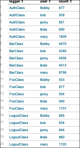
Using the by clause, stats will produce a row per unique value for each field listed, which is similar to the behavior of top. Run the following query:

sourcetype="impl_splunk_gen" error | stats count by logger user

It will produce a table like that shown in the following screenshot:

There are a few things to notice about these results:

1. The results are sorted against the values of the "by" fields, in this case logger followed by user. Unlike top, the largest value will not necessarily be at the top of the list. You can sort...

Using chart to turn data

The chart command is useful for "turning" data across two dimensions. It is useful for both tables and charts. Let's start with one of our examples from stats:

sourcetype="impl_splunk_gen" error | chart count over logger by user

The resulting table looks like this:

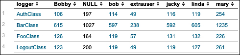
If you look back at the results from stats, the data is presented as one row per combination. Instead of a row per combination, chart generates the intersection of the two fields. You can specify multiple functions, but you may only specify one field each for over and by.

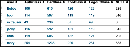
Switching the fields turns the data the other way.

By simply clicking on the chart icon above the table, we can see these results in a chart:

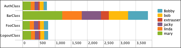
This is a bar chart, with Stack mode set to Stacked, and usenull set to false, like so:

sourcetype="impl_splunk_gen" error
  | chart usenull=false count over logger by user

chart can also be used to simply turn data, even if the data is non-numerical. For example, say we enter this query:

sourcetype="impl_splunk_gen...

Using timechart to show values over time

timechart lets us show numerical values over time. It is similar to the chart command, except that time is always plotted on the x axis. Here are a couple of things to note:

• The events must have an _time field. If you are simply sending the results of a search to timechart, this will always be true. If you are using interim commands, you will need to be mindful of this requirement.

• Time is always "bucketed", meaning that there is no way to draw a point per event.

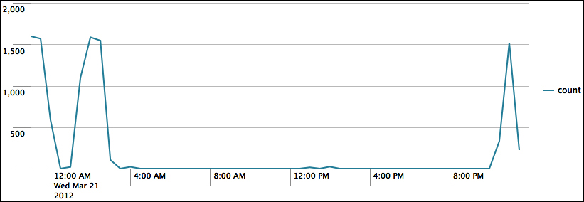
Let's see how many errors have been occurring:

sourcetype="impl_splunk_gen" error | timechart count

The default chart will look something like this:

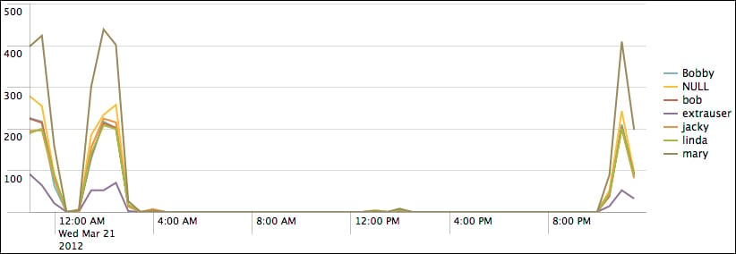
Now let's see how many errors have occurred per user over the same time period. We simply need to add by user to the query:

sourcetype="impl_splunk_gen" error | timechart count by user

This produces the following chart:

As we stated before, the x axis is always time. The y axis can be:

• One or more functions

• A single function with a by clause

• Multiple functions...

Working with fields

All of the fields we have used so far were either indexed fields (such as host, sourcetype, and _time) or fields that were automatically extracted from key=value pairs. Unfortunately, most logs don't follow this format, especially for the first few values in each event. New fields can be created either inline, by using commands, or through configuration.

A regular expression primer

Most of the ways to create new fields in Splunk involve regular expressions. There are many books and sites dedicated to regular expressions, so we will only touch upon the subject here.

Given the log snippet ip=1.2.3.4, let's pull out the subnet (1.2.3) into a new field called subnet. The simplest pattern would be the literal string:

ip=(?P<subnet>1.2.3).4

This is not terribly useful as it will only find the subnet of that one IP address. Let's try a slightly more complicated example:

ip=(?P<subnet>\d+\.\d+\.\d+)\.\d+

Let's step through this pattern:

• ip= simply looks for the raw string...

Summary

This has been a very dense chapter, but we have really just scratched the surface on a number of important topics. In future chapters, we will use these commands and techniques in more and more interesting ways. The possibilities can be a bit dizzying, so we will step through a multitude of examples to illustrate as many scenarios as possible.

In the next chapter, we will build a few dashboards using the wizard-style interfaces provided by Splunk.