Chapter 5
Comparing Models

A map is not the territory it represents, but, if correct, it has a similar structure to the territory. – Alfred Korzybski

Models should be designed as approximations to help us understand a particular problem or a class of related problems. Models are not designed to be verbatim copies of the real world. Thus, all models are wrong in the same sense that maps are not the territory. But not all models are equally wrong; some models will be better than others at describing a given problem.

In the previous chapters, we focused our attention on the inference problem, that is, how to learn the values of parameters from data. In this chapter, we are going to focus on a complementary problem: how to compare two or more models for the same data. As we will learn, this is both a central problem in data analysis and a tricky one. In this chapter, we are going to keep examples super simple, so we can focus on the technical aspects of model comparison. In...

5.1 Posterior predictive checks

We have previously introduced and discussed posterior predictive checks as a way to assess how well a model explains the data used to fit a model. The purpose of this type of testing is not to determine whether a model is incorrect; we already know this! The goal of the exercise is to understand how well we are capturing the data. By performing posterior predictive checks, we aim to better understand the limitations of a model. Once we understand the limitations, we can simply acknowledge them or try to remove them by improving the model. It is expected that a model will not be able to reproduce all aspects of a problem and this is usually not a problem as models are built with a purpose in mind. As different models often capture different aspects of data, we can compare models using posterior predictive checks.

Let’s look at a simple example. We have a dataset with two variables, x and y. We are going to fit these data with a linear model:

We...

5.2 The balance between simplicity and accuracy

When choosing between alternative explanations, there is a principle known as Occam’s razor. In very general terms, this principle establishes that given two or more equivalent explanations for the same phenomenon, the simplest is the preferred explanation. A common criterion of simplicity is the number of parameters in a model.

There are many justifications for this heuristic. We are not going to discuss any of them; we are just going to accept them as a reasonable guide.

Another factor that we generally have to take into account when comparing models is their accuracy, that is, how good a model is at fitting the data. According to this criterion, if we have two (or more) models and one of them explains the data better than the other, then that is the preferred model.

Intuitively, it seems that when comparing models, we tend to prefer those that best fit the data and those that are simple. But what should we do if these two principles...

5.3 Measures of predictive accuracy

”Everything should be made as simple as possible, but not simpler” is a quote often attributed to Einstein. As in a healthy diet, when modeling, we have to maintain a balance. Ideally, we would like to have a model that neither underfits nor overfits the data. We want to somehow balance simplicity and goodness of fit.

In the previous example, it is relatively easy to see that the model of order 0 is too simple, while the model of order 5 is too complex. In order to get a general approach that will allow us to rank models, we need to formalize our intuition about this balance of simplicity and accuracy.

Let’s look at a couple of terms that will be useful to us:

• Within-sample accuracy: The accuracy is measured with the same data used to fit the model.

• Out-of-sample accuracy: The accuracy measured with data not used to fit the model.

The within-sample accuracy will, on average, be greater than the out-of-sample accuracy. That is...

5.4 Calculating predictive accuracy with ArviZ

Fortunately, calculating WAIC and LOO with ArviZ is very simple. We just need to be sure that the Inference Data has the log-likelihood group. When computing a posterior with PyMC, this can be achieved by doing pm.sample(idata_kwargs="log_likelihood": True). Now, let’s see how to compute LOO:

Code 5.3

az.loo(idata_l)

Computed from 8000 posterior samples and 33 observations log-likelihood matrix.

         Estimate       SE elpd_loo   -14.31     2.67
p_loo        2.40        -
------

Pareto k diagnostic values:
                         Count...

5.5 Model averaging

Model selection is attractive for its simplicity, but we might be missing information about uncertainty in our models. This is somewhat similar to calculating the full posterior and then just keeping the posterior mean; this can lead us to be overconfident about what we think we know.

An alternative is to select a single model but to report and analyze the different models together with the values of the calculated information criteria, their standard errors, and perhaps also the posterior predictive checks. It is important to put all these numbers and tests in the context of our problem so that we and our audience can get a better idea of the possible limitations and shortcomings of the models. For those working in academia, these elements can be used to add elements to the discussion section of a paper, presentation, thesis, etc. In industry, this can be useful for informing stakeholders about the advantages and limitations of models, predictions, and conclusions...

5.6 Bayes factors

An alternative to LOO, cross-validation, and information criteria is Bayes factors. It is common for Bayes factors to show up in the literature as a Bayesian alternative to frequentist hypothesis testing.

The Bayesian way of comparing k models is to calculate the marginal likelihood of each model p(y|M_k), i.e., the probability of the observed data Y given the model M_k. The marginal likelihood is the normalization constant of Bayes’ theorem. We can see this if we write Bayes’ theorem and make explicit the fact that all inferences depend on the model.

where, y is the data, θ is the parameters, and M_k is a model out of k competing models.

If our main objective is to choose only one model, the best from a set of models, we can choose the one with the largest value of p(y|M_k). This is fine if we assume that all models have the same prior probability. Otherwise, we must calculate:

If, instead, our main objective is to compare models to determine which...

5.7 Bayes factors and inference

So far, we have used Bayes factors to judge which model seems to be better at explaining the data, and we found that one of the models is ≈ 5 times better than the other.

But what about the posterior we get from these models? How different are they? Table 5.2 summarizes these two posteriors:

	mean	sd	hdi_3%	hdi_97%
uniform	0.5	0.05	0.4	0.59
peaked	0.5	0.04	0.42	0.57

Table 5.2: Statistics for the models with uniform and peaked priors computed using the ArviZ summary function

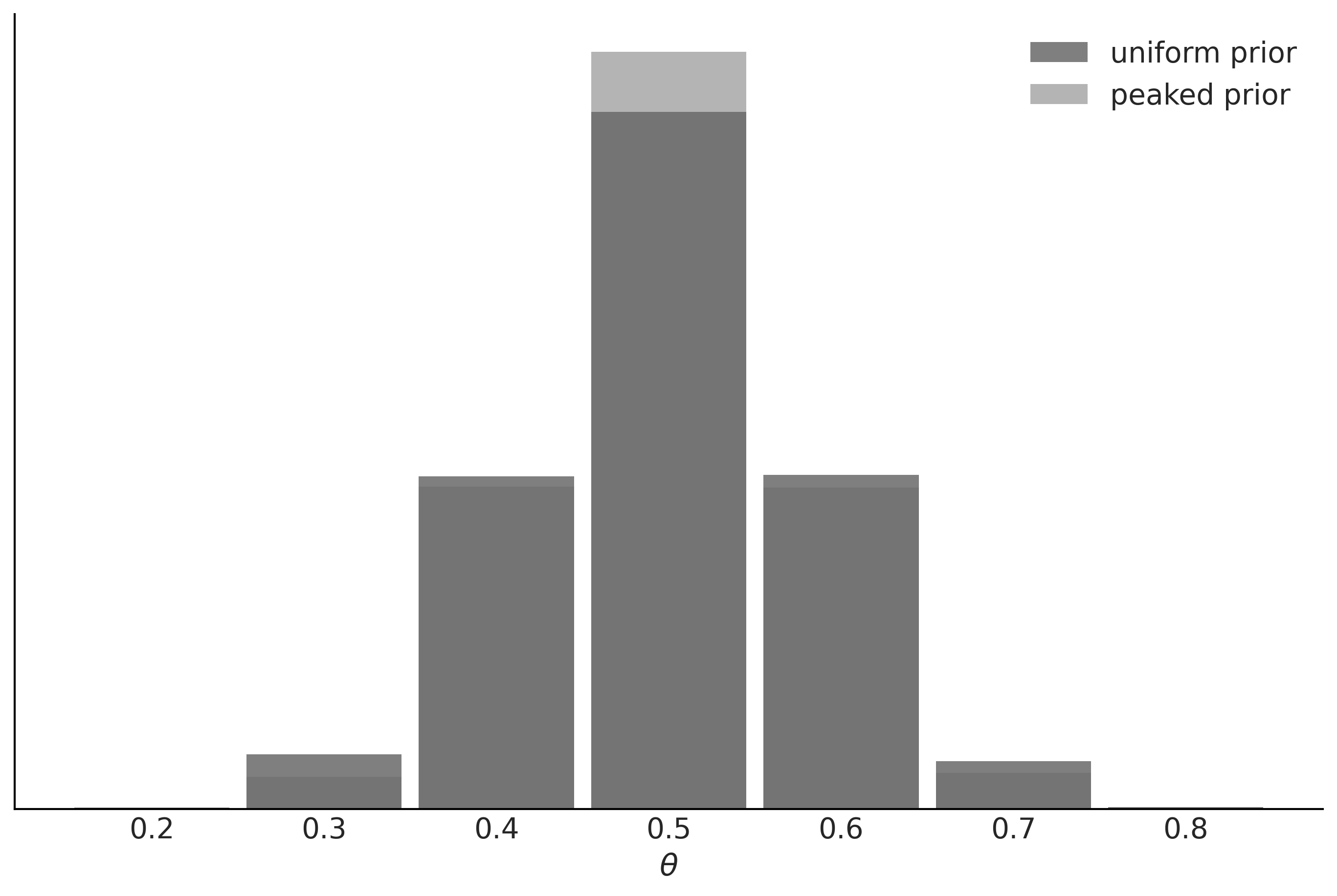
We can argue that the results are quite similar; we have the same mean value for θ and a slightly wider posterior for model_0, as expected since this model has a wider prior. We can also check the posterior predictive distribution to see how similar they are (see Figure 5.13).

Figure 5.13: Posterior predictive distributions for models with uniform and peaked priors

In this example, the observed data is more consistent with model_1, because the prior...

5.8 Regularizing priors

Using informative and weakly informative priors is a way of introducing bias in a model and, if done properly, this can be really good because bias prevents overfitting and thus contributes to models being able to make predictions that generalize well. This idea of adding a bias element to reduce generalization errors without affecting the ability of the model to adequately model a problem is known as regularization. This regularization often takes the form of a term penalizing certain values for the parameters in a model, like too-big coefficients in a regression model. Restricting parameter values is a way of reducing the data a model can represent, thus reducing the chances that a model will capture noise instead of the signal.

This regularization idea is so powerful and useful that it has been discovered several times, including outside the Bayesian framework. For regression models, and outside Bayesian statistics, two popular regularization methods are ridge...

5.9 Summary

In this chapter, we have seen how to compare models using posterior predictive checks, information criteria, approximated cross-validation, and Bayes factors.

Posterior predictive check is a general concept and practice that can help us understand how well models are capturing different aspects of the data. We can perform posterior predictive checks with just one model or with many models, and thus we can use it as a method for model comparison. Posterior predictive checks are generally done via visualizations, but numerical summaries like Bayesian values can also be helpful.

Good models have a good balance between complexity and predictive accuracy. We exemplified this feature by using the classical example of polynomial regression. We discussed two methods to estimate the out-of-sample accuracy without leaving data aside: cross-validation and information criteria. From a practical point of view, information criteria is a family of theoretical methods looking to balance two...

5.10 Exercises

1. This exercise is about regularization priors. In the code that generates the x_c, y_c data (see https://github.com/aloctavodia/BAP3), change order=2 to another value, such as order=5. Then, fit model_q and plot the resulting curve. Repeat this, but now using a prior for β with sd=100 instead of sd=1 and plot the resulting curve. How do the curves differ? Try this out with sd=np.array([10, 0.1, 0.1, 0.1, 0.1]), too.

2. Repeat the previous exercise but increase the amount of data to 500 data points.

3. Fit a cubic model (order 3), compute WAIC and LOO, plot the results, and compare them with the linear and quadratic models.

4. Use pm.sample_posterior_predictive() to rerun the PPC example, but this time, plot the values of y instead of the values of the mean.

5. Read and run the posterior predictive example from PyMC’s documentation at https://www.pymc.io/projects/docs/en/stable/learn/core_notebooks/posterior_predictive.html. Pay special attention to the use of...

Join our community Discord space

Join our Discord community to meet like-minded people and learn alongside more than 5000 members at: https://packt.link/bayesian