Reader small image

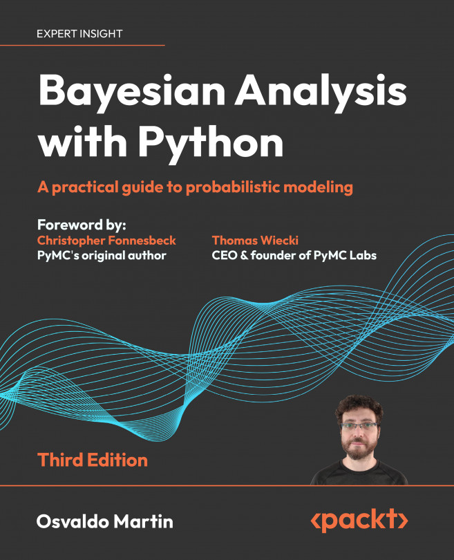
You're reading from  Bayesian Analysis with Python - Third Edition

Product typeBook
Published inJan 2024
Reading LevelExpert
PublisherPackt
ISBN-139781805127161
Edition3rd Edition
Languages
Right arrow
Author (1)
Osvaldo Martin
Osvaldo Martin
author image
Osvaldo Martin

Osvaldo Martin is a researcher at CONICET, in Argentina. He has experience using Markov Chain Monte Carlo methods to simulate molecules and perform Bayesian inference. He loves to use Python to solve data analysis problems. He is especially motivated by the development and implementation of software tools for Bayesian statistics and probabilistic modeling. He is an open-source developer, and he contributes to Python libraries like PyMC, ArviZ and Bambi among others. He is interested in all aspects of the Bayesian workflow, including numerical methods for inference, diagnosis of sampling, evaluation and criticism of models, comparison of models and presentation of results.
Read more about Osvaldo Martin

Right arrow

Chapter 8
Gaussian Processes

Lonely? You have yourself. Your infinite selves. - Rick Sanchez (at least the one from dimension C-137)

In the last chapter, we learned about the Dirichlet process, an infinite-dimensional generalization of the Dirichlet distribution that can be used to set a prior on an unknown continuous distribution. In this chapter, we will learn about the Gaussian process, an infinite-dimensional generalization of the Gaussian distribution that can be used to set a prior on unknown functions. Both the Dirichlet process and the Gaussian process are used in Bayesian statistics to build flexible models where the number of parameters is allowed to increase with the size of the data.

We will cover the following topics:

  • Functions as probabilistic objects

  • Kernels

  • Gaussian processes with Gaussian likelihoods

  • Gaussian processes with non-Gaussian likelihoods

  • Hilbert space Gaussian process

8.1 Linear models and non-linear data

In Chapter 4 and Chapter 6 we learned how to build models of the general form:

θ = 𝜓 (ϕ(X )𝛽 )

Here, θ is a parameter for some probability distribution, for example, the mean of a Gaussian, the p parameter of the binomial, the rate of a Poisson, and so on. We call the inverse link function and is some other function we use to potentially transform the data, like a square root, a polynomial function, or something else.

Fitting, or learning, a Bayesian model can be seen as finding the posterior distribution of the weights β, and thus this is known as the weight view of approximating functions. As we already saw with polynomial and splines regression, by letting be a non-linear function, we can map the inputs onto a feature space. We also saw that by using a polynomial of the proper degree, we can perfectly fit any function. But unless we apply some form of regularization, for example, using prior distributions, this will lead to models that memorize...

8.2 Modeling functions

We will begin our discussion of Gaussian processes by first describing a way to represent functions as probabilistic objects. We may think of a function f as a mapping from a set of inputs X to a set of outputs Y . Thus, we can write:

Y = f(X )

One very crude way to represent functions is by listing for each xi value its corresponding yi value as in Table 8.1. You may remember this way of representing functions from elementary school.

x y
0.00 0.46
0.33 2.60
0.67 5.90
1.00 7.91

Table 8.1: A tabular representation of a function (sort of)

As a general case, the values of X and Y will live on the real line; thus, we can see a function as a (potentially) infinite and ordered list of paired values (xi,yi). The order is important because, if we shuffle the values, we will get different functions.

Following this description, we can represent, numerically, any specific function we want. But what if we want to represent functions probabilistically? Well,...

8.3 Multivariate Gaussians and functions

In Figure 8.1, we represented a function as a collection of samples from 1-dimensional Gaussian distributions. One alternative is to use an n-dimensional multivariate Gaussian distribution to get a sample vector of length n. Actually, you may want to try to reproduce Figure 8.1 but replacing np.random.normal(0, 1, len(x)) with np.random.multivariate_normal, with a mean of np.zeros_like(x) and a standard deviation of np.eye(len(x). The advantage of working with a Multivariate Normal is that we can use the covariance matrix to encode information about the function. For instance, by setting the covariance matrix to np.eye(len(x)), we are saying that each of the 10 points, where we are evaluating the function, has a variance of 1. We are also saying that the variance between them, that is, their covariances, is 0. In other words, they are independent. If we replace those zeros with other numbers, we could get covariances telling a different story...

8.4 Gaussian processes

Now we are ready to understand what Gaussian processes (GPs) are and how they are used in practice. A somewhat formal definition of GPs, taken from Wikipedia, is as follows:

”The collection of random variables indexed by time or space, such that every finite collection of those random variables has a MultivariateNormal distribution, i.e. every finite linear combination of them is normally distributed.”

This is probably not a very useful definition, at least not at this stage of your learning path. The trick to understanding Gaussian processes is to realize that the concept of GP is a mental (and mathematical) scaffold, since, in practice, we do not need to directly work with this infinite mathematical object. Instead, we only evaluate the GPs at the points where we have data. By doing this, we collapse the infinite-dimensional GP into a finite multivariate Gaussian distribution with as many dimensions as data points. Mathematically, this collapse...

8.5 Gaussian process regression

Let’s assume we can model a variable Y as a function f of X plus some Gaussian noise:

Y ∼ 𝒩 (μ = f(X ),σ = 𝜖)

If f is a linear function of X, then this assumption is essentially the same one we used in Chapter 4 when we discussed simple linear regression. In this chapter, instead, we are going to use a more general expression for f by setting a prior over it. In that way, we will be able to get more complex functions than linear. If we decided to use Gaussian processes as this prior, then we can write:

 ′ f(X ) = 𝒢𝒫 (μX,𝜅(X, X ))

Here, represents a Gaussian process with the mean function μX and covariance function K(X,X). Even though in practice, we always work with finite objects, we used the word function to indicate that mathematically, the mean and covariance are infinite objects.

I mentioned before that working with Gaussians is nice. For instance, if the prior distribution is a GP and the likelihood is a Gaussian distribution, then the posterior is also a GP and we can...

8.6 Gaussian process regression with PyMC

The gray line in Figure 8.4 is a sin function. We are going to assume we don’t know this function and instead, all we have is a set of data points (dots). Then we use a Gaussian process to approximate the function that generated those data points.

PIC

Figure 8.4: Synthetic data (dots) generated from a known function (line)

GPs are implemented in PyMC as a series of Python classes that deviate a little bit from what we have seen in previous models; nevertheless, the code is still very PyMConic. I have added a few comments in the following code to guide you through the key steps of defining a GP with PyMC.

Code 8.3

# A one-dimensional column vector of inputs. 
X = x[:, None] 
 
with pm.Model() as model_reg: 
    # hyperprior for lengthscale kernel parameter 
    ℓ = pm.InverseGamma("ℓ", 7, 17) 
    # instanciate...

8.7 Gaussian process classification

In Chapter 4, we saw how a linear model can be used to classify data. We used a Bernoulli likelihood with a logistic inverse link function. Then, we applied a boundary decision rule. In this section, we are going to do the same, but this time using a GP instead of a linear model. As we did with model_lrs from Chapter 4, we are going to use the iris dataset with two classes, setosa and versicolor, and one predictor variable, the sepal length.

For this model, we cannot use the pm.gp.Marginal class, because that class is restricted to Gaussian likelihoods as it takes advantage of the mathematical tractability of the combination of a GP prior with a Gaussian likelihood. Instead, we need to use the more general class pm.gp.Latent.

Code 8.7

with pm.Model() as model_iris: 
    ℓ = pm.InverseGamma('ℓ', *get_ig_params(x_1)) 
    cov = pm.gp.cov.ExpQuad(1, ℓ) 
&...

8.8 Cox processes

Now we are going to model count data. We will see two examples; one with a time-varying rate and one with a 2D spatially varying rate. To do this, we will use a Poisson likelihood and the rate will be modeled using a Gaussian process. Because the rate of the Poisson distribution is limited to positive values, we will use an exponential as the inverse link function, as we did for the NegativeBinomial regression from Chapter 4.

We can think of a Poisson process as a distribution over collections of points in a given space where every finite collection of those random variables has a Poisson distribution. When the rate of the Poisson process is itself a stochastic process, such as, for example, a Gaussian process, then we have a Cox process.

8.8.1 Coal mining disasters

The first example is known as the coal mining disasters. This example consists of a record of coal-mining disasters in the UK from 1851 to 1962. The number of disasters is thought to have been affected...

8.9 Regression with spatial autocorrelation

The following example is taken from Statistical Rethinking: A Bayesian Course with Examples in R and STAN, Second Edition by Richard McElreath, Copyright (2020) by Chapman and Hall/CRC. Reproduced by permission of Taylor & Francis Group. I strongly recommend reading this book, as you will find many good examples like this and very good explanations. The only caveat is that the book examples are in R/Stan, but don’t worry and keep sampling; you will find the Python/PyMC version of those examples in the https://github.com/pymc-devs/pymc-resources resources.

For this example we have 10 different island societies; for each one of them, we have the number of tools they use. Some theories predict that larger populations develop and sustain more tools than smaller populations. Thus, we have a regression problem where the dependent variable is the number of tools and the independent variable is the population. Because the number of tools...

8.10 Hilbert space GPs

Gaussian processes can be slow. The main reason is that their computation requires us to invert a matrix, whose size grows with the number of observations. This operation is computationally costly and does not scale very nicely. For that reason, a large portion of the research around GPs has been to find approximations to compute them faster and allow scaling them to large data.

We are going to discuss only one of those approximations, namely the Hilbert Space Gaussian Process (HSGP), without going into the details of how this approximation is achieved. Conceptually, we can think of it as a basis function expansion similar, in spirit, to how splines are constructed (see Chapter 6). The consequence of this approximation is that it turns the matrix inversion into just matrix multiplication, a much faster operation.

But When Will It Work?

We can only use HSGPs for low dimensions (1 to maybe 3 or 4), and only for some kernels like the exponential quadratic or Matern...

8.11 Summary

A Gaussian process is a generalization of the multivariate Gaussian distribution to infinitely many dimensions and is fully specified by a mean function and a covariance function. Since we can conceptually think of functions as infinitely long vectors, we can use Gaussian processes as priors over functions. In practice, we do not work with infinite objects but with multivariate Gaussian distributions with as many dimensions as data points. To define their corresponding covariance function, we used properly parameterized kernels; and by learning about those hyperparameters, we ended up learning about arbitrary complex functions.

In this chapter, we have given a short introduction to GPs. We have covered regression, semi-parametric models (the islands example), combining two or more kernels to better describe the unknown function, and how a GP can be used for classification tasks. There are many other topics we could have discussed. Nevertheless, I hope this introduction to...

8.12 Exercises

  1. For the example in the Covariance functions and kernels section, make sure you understand the relationship between the input data and the generated covariance matrix. Try using other input such as data = np.random.normal(size=4).

  2. Rerun the code generating Figure 8.3 and increase the number of samples obtained from the GP prior to around 200. In the original figure, the number of samples is 2. What is the range of the generated values?

  3. For the generated plot in the previous exercise, compute the standard deviation for the values at each point. Do this in the following form:

    • Visually, just observing the plots

    • Directly from the values generated from pz.MVNormal(.).rvs

    • By inspecting the covariance matrix (if you have doubts go back to exercise 1)

    Did the values you get from these three methods match?

  4. Use test points np.linspace(np.floor(x.min()), 20, 100)[:,None] and re-run model_reg. Plot the results. What did you observe? How is this related to the specification...

Join our community Discord space

Join our Discord community to meet like-minded people and learn alongside more than 5000 members at: https://packt.link/bayesian

PIC

lock icon
The rest of the chapter is locked
You have been reading a chapter from
Bayesian Analysis with Python - Third Edition
Published in: Jan 2024Publisher: PacktISBN-13: 9781805127161
Register for a free Packt account to unlock a world of extra content!
A free Packt account unlocks extra newsletters, articles, discounted offers, and much more. Start advancing your knowledge today.
undefined
Unlock this book and the full library FREE for 7 days
Get unlimited access to 7000+ expert-authored eBooks and videos courses covering every tech area you can think of
Renews at $15.99/month. Cancel anytime

Author (1)

author image
Osvaldo Martin

Osvaldo Martin is a researcher at CONICET, in Argentina. He has experience using Markov Chain Monte Carlo methods to simulate molecules and perform Bayesian inference. He loves to use Python to solve data analysis problems. He is especially motivated by the development and implementation of software tools for Bayesian statistics and probabilistic modeling. He is an open-source developer, and he contributes to Python libraries like PyMC, ArviZ and Bambi among others. He is interested in all aspects of the Bayesian workflow, including numerical methods for inference, diagnosis of sampling, evaluation and criticism of models, comparison of models and presentation of results.
Read more about Osvaldo Martin