Reader small image

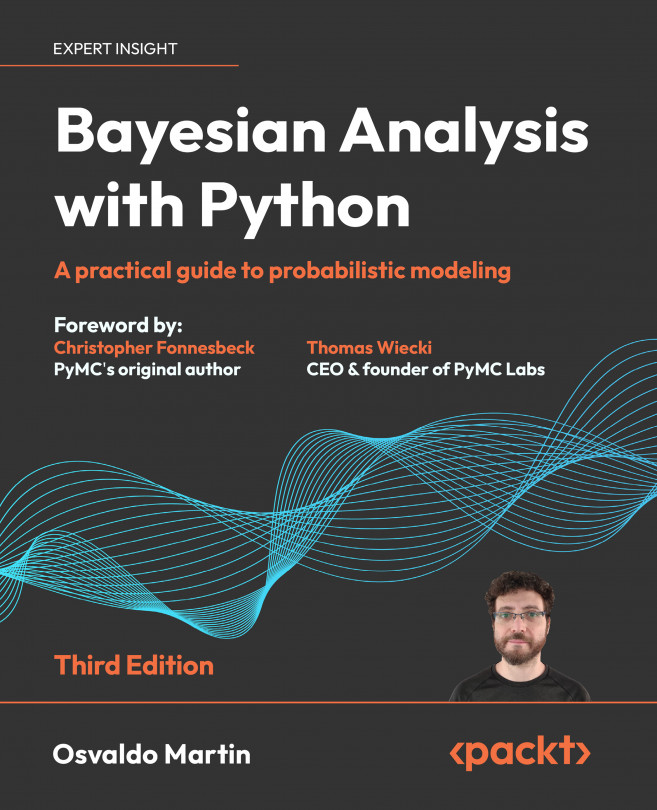
You're reading from  Bayesian Analysis with Python - Third Edition

Product typeBook
Published inJan 2024
Reading LevelExpert
PublisherPackt
ISBN-139781805127161
Edition3rd Edition
Languages
Right arrow
Author (1)
Osvaldo Martin
Osvaldo Martin
author image
Osvaldo Martin

Osvaldo Martin is a researcher at CONICET, in Argentina. He has experience using Markov Chain Monte Carlo methods to simulate molecules and perform Bayesian inference. He loves to use Python to solve data analysis problems. He is especially motivated by the development and implementation of software tools for Bayesian statistics and probabilistic modeling. He is an open-source developer, and he contributes to Python libraries like PyMC, ArviZ and Bambi among others. He is interested in all aspects of the Bayesian workflow, including numerical methods for inference, diagnosis of sampling, evaluation and criticism of models, comparison of models and presentation of results.
Read more about Osvaldo Martin

Right arrow

Chapter 2
Programming Probabilistically

Our golems rarely have a physical form, but they too are often made of clay living in silicon as computer code. – Richard McElreath

Now that we have a very basic understanding of probability theory and Bayesian statistics, we are going to learn how to build probabilistic models using computational tools. Specifically, we are going to learn about probabilistic programming with PyMC [Abril-Pla et al.2023]. The basic idea is that we use code to specify statistical models and then PyMC will solve those models for us. We will not need to write Bayes’ theorem in explicit form. This is a good strategy for two reasons. First, many models do not lead to an analytic closed form, and thus we can only solve those models using numerical techniques. Second, modern Bayesian statistics is mainly done by writing code. We will be able to see that probabilistic programming offers an effective way to build and solve complex models and...
2.1 Probabilistic programming

Bayesian statistics is conceptually very simple. We have the knowns and the unknowns, and we use Bayes’ theorem to condition the latter on the former. If we are lucky, this process will reduce the uncertainty about the unknowns. Generally, we refer to the knowns as data and treat it like constants, and the unknowns as parameters and treat them as random variables.

Although conceptually simple, fully probabilistic models often lead to analytically intractable expressions. For many years, this was a real problem and one of the main issues that hindered the adoption of Bayesian methods beyond some niche applications. The arrival of the computational era and the development of numerical methods that, at least in principle, can be used to solve any inference problem, have dramatically transformed the Bayesian data analysis practice. We can think of these numerical methods as universal inference engines. The possibility of automating the inference process...

2.2 Summarizing the posterior

Generally, the first task we will perform after sampling from the posterior is to check what the results look like. The plot_trace function from ArviZ is ideally suited to this task:

Code 2.3

az.plot_trace(idata)
PIC

Figure 2.1: A trace plot for the posterior of our_first_model

Figure 2.1 shows the default result when calling az.plot_trace; we get two subplots for each unobserved variable. The only unobserved variable in our model is θ. Notice that y is an observed variable representing the data; we do not need to sample that because we already know those values. Thus we only get two subplots. On the left, we have a Kernel Density Estimation (KDE) plot; this is like the smooth version of the histogram. Ideally, we want all chains to have a very similar KDE, like in Figure 2.1. On the right, we get the individual values at each sampling step; we get as many lines as chains. Ideally, we want it to be something that looks noisy, with no clear...

2.3 Posterior-based decisions

Sometimes, describing the posterior is not enough. We may need to make decisions based on our inferences and reduce a continuous estimation to a dichotomous one: yes-no, healthy-sick, contaminated-safe, and so on. For instance, is the coin fair? A fair coin is one with a θ value of exactly 0.5. We can compare the value of 0.5 against the HDI interval. From Figure 2.3, we can see that the HDI goes from 0.03 to 0.7 and hence 0.5 is included in the HDI. We can interpret this as an indication that the coin may be tail-biased, but we cannot completely rule out the possibility that the coin is actually fair. If we want a sharper decision, we will need to collect more data to reduce the spread of the posterior, or maybe we need to find out how to define a more informative prior.

2.3.1 Savage-Dickey density ratio

One way to evaluate how much support the posterior provides for a given value is to compare the ratio of the posterior and prior densities at...

2.4 Gaussians all the way down

Gaussians are very appealing from a mathematical point of view. Working with them is relatively easy, and many operations applied to Guassians return another Gaussian. Additionally, many natural phenomena can be nicely approximated using Gaussians; essentially, almost every time that we measure the average of something, using a big enough sample size, that average will be distributed as a Gaussian. The details of when this is true, when this is not true, and when this is more or less true, are elaborated in the central limit theorem (CLT); you may want to stop reading now and search about this really central statistical concept (terrible pun intended).

Well, we were saying that many phenomena are indeed averages. Just to follow a cliché, the height (and almost any other trait of a person, for that matter) is the result of many environmental factors and many genetic factors, and hence we get a nice Gaussian distribution for the height of adult people...

2.5 Posterior predictive checks

One of the nice elements of the Bayesian toolkit is that once we have a posterior p(θ|Y ), it is possible to use it to generate predictions p(). Mathematically, this can be done by computing:

 ∫ p(˜Y | Y ) = p(˜Y | θ) p(θ | Y )dθ

This distribution is known as the posterior predictive distribution. It is predictive because it is used to make predictions, and posterior because it is computed using the posterior distribution. So we can think of this as the distribution of future data given the model, and observed data.

Using PyMC is easy to get posterior predictive samples; we don’t need to compute any integral. We just need to call the sample_posterior_predictive function and pass the InferenceData object as the first argument. We also need to pass the model object, and we can use the extend_inferencedata argument to add the posterior predictive samples to the InferenceData object. The code is:

Code 2.14

pm.sample_posterior_predictive(idata_g, model=model_g, ...

2.6 Robust inferences

One objection we may have with model_g is that we are assuming a Normal distribution, but we have two data points away from the bulk of the data. By using a Normal distribution for the likelihood, we are indirectly assuming that we are not expecting to see a lot of data points far away from the bulk. Figure 2.13 shows the result of combining these assumptions with the data. Since the tails of the Normal distribution fall quickly as we move away from the mean, the Normal distribution (at least an anthropomorphized one) is surprised by seeing those two points and reacts in two ways, moving its mean towards those points and increasing its standard deviation. Another intuitive way of interpreting this is by saying that those points have an excessive weight in determining the parameters of the Normal distribution.

So, what can we do? One option is to check for errors in the data. If we retrace our steps we may find an error in the code while cleaning or preprocessing...

2.7 InferenceData

InferenceData is a rich container for the results of Bayesian inference. A modern Bayesian analysis potentially generates many sets of data including posterior samples and posterior predictive samples. But we also have observed data, samples from the prior, and even statistics generated by the sampler. All this data, and more, can be stored in an InferenceData object. To help keep all this information organized, each one of these sets of data has its own group. For instance, the posterior samples are stored in the posterior group. The observed data is stored in the observed_data group.

Figure 2.18 shows an HTML representation of the InferenceData for model_g. We can see 4 groups: posterior, posterior_predictive, sample_stats, and observed_data. All of them are collapsed except for the posterior group. We can see we have two coordinates chain and draw of dimensions 4 and 1000 respectively. We also have 2 variables μ and σ.

PIC

Figure 2.18: InferenceData...

2.8 Groups comparison

One pretty common statistical analysis is group comparison. We may be interested in how well patients respond to a certain drug, the reduction of car accidents by the introduction of new traffic regulations, student performance under different teaching approaches, and so on. Sometimes, this type of question is framed under the hypothesis testing scenario and the goal is to declare a result statistically significant. Relying only on statistical significance can be problematic for many reasons: on the one hand, statistical significance is not equivalent to practical significance; on the other hand, a really small effect can be declared significant just by collecting enough data.

The idea of hypothesis testing is connected to the concept of p-values. This is not a fundamental connection but a cultural one; people are used to thinking that way mostly because that’s what they learn in most introductory statistical courses. There is a long record of studies and...

2.9 Summary

Although Bayesian statistics is conceptually simple, fully probabilistic models often lead to analytically intractable expressions. For many years, this was a huge barrier, hindering the wide adoption of Bayesian methods. Fortunately, maths, statistics, physics, and computer science came to the rescue in the form of numerical methods that are capable—at least in principle—of solving any inference problem. The possibility of automating the inference process has led to the development of probabilistic programming languages, allowing a clear separation between model definition and inference. PyMC is a Python library for probabilistic programming with a very simple, intuitive, and easy-to-read syntax that is also very close to the statistical syntax used to describe probabilistic models.

We introduced the PyMC library by revisiting the coin-flip model from Chapter 1, this time without analytically deriving the posterior. PyMC models are defined inside a context manager...

2.10 Exercises

  1. Using PyMC, change the parameters of the prior Beta distribution in our_first_model to match those of the previous chapter. Compare the results to the previous chapter.

  2. Compare the model our_first_model with prior θ Beta(1,1) with a model with prior θ (0,1). Are the posteriors similar or different? Is the sampling slower, faster, or the same? What about using a Uniform over a different interval such as [-1, 2]? Does the model run? What errors do you get?

  3. PyMC has a function pm.model_to_graphviz that can be used to visualize the model. Use it to visualize the model our_first_model. Compare the result with the Kruschke diagram. Use pm.model_to_graphviz to visualize model comparing_groups.

  4. Read about the coal mining disaster model that is part of the PyMC documentation ( https://shorturl.at/hyCX2). Try to implement and run this model by yourself.

  5. Modify model_g, change the prior for the mean to a Gaussian distribution centered at the...

Join our community Discord space

Join our Discord community to meet like-minded people and learn alongside more than 5000 members at: https://packt.link/bayesian

PIC

lock icon
The rest of the chapter is locked
You have been reading a chapter from
Bayesian Analysis with Python - Third Edition
Published in: Jan 2024Publisher: PacktISBN-13: 9781805127161
Register for a free Packt account to unlock a world of extra content!
A free Packt account unlocks extra newsletters, articles, discounted offers, and much more. Start advancing your knowledge today.
undefined
Unlock this book and the full library FREE for 7 days
Get unlimited access to 7000+ expert-authored eBooks and videos courses covering every tech area you can think of
Renews at $15.99/month. Cancel anytime

Author (1)

author image
Osvaldo Martin

Osvaldo Martin is a researcher at CONICET, in Argentina. He has experience using Markov Chain Monte Carlo methods to simulate molecules and perform Bayesian inference. He loves to use Python to solve data analysis problems. He is especially motivated by the development and implementation of software tools for Bayesian statistics and probabilistic modeling. He is an open-source developer, and he contributes to Python libraries like PyMC, ArviZ and Bambi among others. He is interested in all aspects of the Bayesian workflow, including numerical methods for inference, diagnosis of sampling, evaluation and criticism of models, comparison of models and presentation of results.
Read more about Osvaldo Martin