

Introducing Pandas DataFrames
Pandas is an open source library used for data analysis and manipulation. It provides various functions for data wrangling, cleaning, and merging operations. Let us see how to explore data using the pandas library. For this, we will use the Income dataset located on GitHub and explore it to find the following insights:
- How many unique values are there for age, education, and profession in the Income dataset? What are the observations for each unique age?
- Summary statistics such as mean value and quantile values for each feature. What is the average age of the adult for the income range > $50K?
- How is income dependent on independent variables such as age, education, and profession using bivariate analysis?
Let us first read the data into a DataFrame using the pandas library.
A DataFrame is a structure that represents two-dimensional data with columns and rows, and it is similar to a SQL table. To get started, ensure that you create the requirements.txt file and add the required Python libraries as follows:
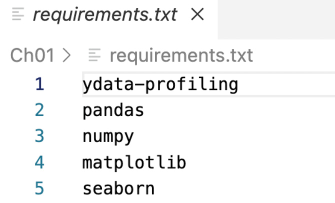
Figure 1.2 – Contents of the requirements.txt file
Next, run the following command from your Python notebook cell to install the libraries added in the requirements.txt file:
%pip install -r requirements.txt
Now, let’s import the required Python libraries using the following import statements:
# import libraries for loading dataset
import pandas as pd
import numpy as np
# import libraries for plotting
import matplotlib.pyplot as plt
import seaborn as sns
from matplotlib import rcParams
%matplotlib inline
plt.style.use('dark_background')
# ignore warnings
import warnings
warnings.filterwarnings('ignore')
Next, in the following code snippet, we are reading the adult_income.csv file and writing to the DataFrame (df):
# loading the dataset
df = pd.read_csv("<your file path>/adult_income.csv", encoding='latin-1)'
Now the data is loaded to df.
Let us see the size of the DataFrame using the following code snippet:
df.shape
We will see the shape of the DataFrame as a result:
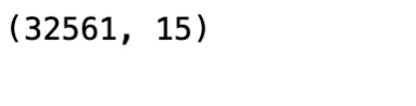
Figure 1.3 – Shape of the DataFrame
So, we can see that there are 32,561 observations (rows) and 15 features (columns) in the dataset.
Let us print the 15 column names in the dataset:
df.columns
We get the following result:
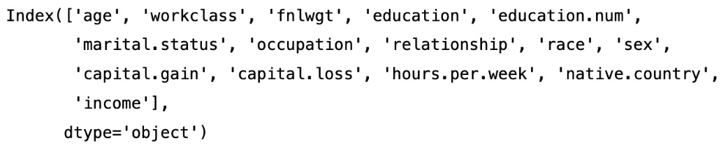
Figure 1.4 – The names of the columns in our dataset
Now, let’s see the first five rows of the data in the dataset with the following code:
df.head()
We can see the output in Figure 1.5:
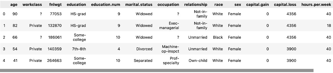
Figure 1.5 – The first five rows of data
Let’s see the last five rows of the dataset using tail, as shown in the following figure:
df.tail()
We will get the following output.
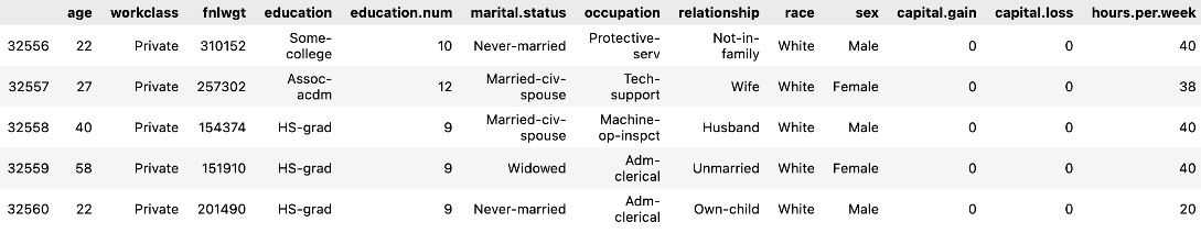
Figure 1.6 – The last five rows of data
As we can see, education and education.num are redundant columns, as education.num is just the ordinal representation of the education column. So, we will remove the redundant education.num column from the dataset as one column is enough for model training. We will also drop the race column from the dataset using the following code snippet as we will not use it here:
# As we observe education and education.num both are the same , so we can drop one of the columns
df.drop(['education.num'], axis = 1, inplace = True)
df.drop(['race'], axis = 1, inplace = True)
Here, axis = 1 refers to the columns axis, which means that you are specifying that you want to drop a column. In this case, you are dropping the columns labeled education.num and race from the DataFrame.
Now, let’s print the columns using info() to make sure the race and education.num columns are dropped from the DataFrame:
df.info()
We will see the following output:
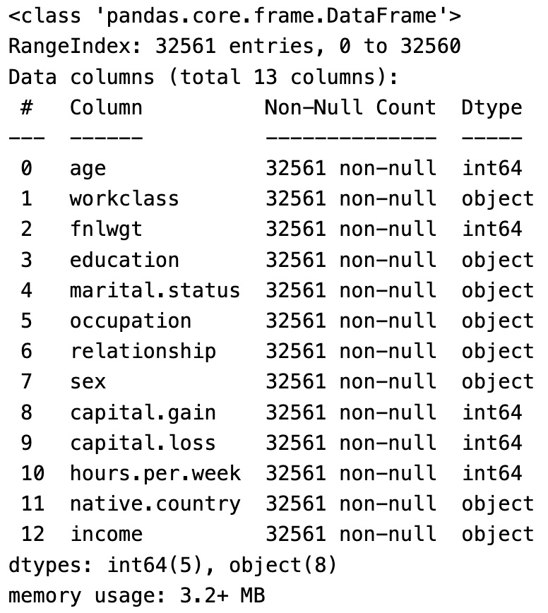
Figure 1.7 – Columns in the DataFrame
We can see in the preceding data there are now only 13 columns as we deleted 2 of them from the previous total of 15 columns.
In this section, we have seen what a Pandas DataFrame is and loaded a CSV dataset into one. We also saw the various columns in the DataFrame and their data types. In the following section, we will generate the summary statistics for the important features using Pandas.