Statistics is the branch of mathematics dealing with the collection, analysis, interpretation, presentation, and organization of numerical data.
Statistical modeling is applying statistics on data to find underlying hidden relationships by analyzing the significance of the variables.
Statistical fundamentals and terminology for model building and validation
Statistics itself is a vast subject on which a complete book could be written; however, here the attempt is to focus on key concepts that are very much necessary with respect to the machine learning perspective. In this section, a few fundamentals are covered and the remaining concepts will be covered in later chapters wherever it is necessary to understand the statistical equivalents of machine learning.
Predictive analytics depends on one major assumption: that history repeats itself!
By fitting a predictive model on historical data after validating key measures, the same model will be utilized for predicting future events based on the same explanatory variables that were significant on past data.
The first movers of statistical model implementers were the banking and pharmaceutical industries; over a period, analytics expanded to other industries as well.
Statistical models are a class of mathematical models that are usually specified by mathematical equations that relate one or more variables to approximate reality. Assumptions embodied by statistical models describe a set of probability distributions, which distinguishes it from non-statistical, mathematical, or machine learning models
Statistical models always start with some underlying assumptions for which all the variables should hold, then the performance provided by the model is statistically significant. Hence, knowing the various bits and pieces involved in all building blocks provides a strong foundation for being a successful statistician.
In the following section, we have described various fundamentals with relevant codes:
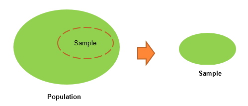
- Population: This is the totality, the complete list of observations, or all the data points about the subject under study.
- Sample: A sample is a subset of a population, usually a small portion of the population that is being analyzed.
Note
Usually, it is expensive to perform an analysis on an entire population; hence, most statistical methods are about drawing conclusions about a population by analyzing a sample.
- Parameter versus statistic: Any measure that is calculated on the population is a parameter, whereas on a sample it is called a statistic.
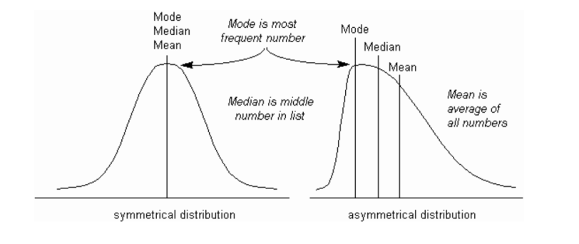
- Mean: This is a simple arithmetic average, which is computed by taking the aggregated sum of values divided by a count of those values. The mean is sensitive to outliers in the data. An outlier is the value of a set or column that is highly deviant from the many other values in the same data; it usually has very high or low values.
- Median: This is the midpoint of the data, and is calculated by either arranging it in ascending or descending order. If there are N observations.
- Mode: This is the most repetitive data point in the data:
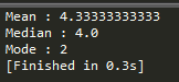
The Python code for the calculation of mean, median, and mode using a numpy array and the stats package is as follows:
>>> import numpy as np
>>> from scipy import stats

>>> data = np.array([4,5,1,2,7,2,6,9,3])

# Calculate Mean
>>> dt_mean = np.mean(data) ; print ("Mean :",round(dt_mean,2))

# Calculate Median
>>> dt_median = np.median(data) ; print ("Median :",dt_median)

# Calculate Mode
>>> dt_mode =  stats.mode(data); print ("Mode :",dt_mode[0][0])
The output of the preceding code is as follows:
Note
We have used a NumPy array instead of a basic list as the data structure; the reason behind using this is the scikit-learn package built on top of NumPy array in which all statistical models and machine learning algorithms have been built on NumPy array itself. The mode function is not implemented in the numpy package, hence we have used SciPy's stats package. SciPy is also built on top of NumPy arrays.
The R code for descriptive statistics (mean, median, and mode) is given as follows:
data <- c(4,5,1,2,7,2,6,9,3)
dt_mean = mean(data) ; print(round(dt_mean,2))
dt_median = median (data); print (dt_median)

func_mode <- function (input_dt) {
  unq <- unique(input_dt)  unq[which.max(tabulate(match(input_dt,unq)))]
}

dt_mode = func_mode (data); print (dt_mode)
Note
We have used the default stats package for R; however, the mode function was not built-in, hence we have written custom code for calculating the mode.
- Measure of variation: Dispersion is the variation in the data, and measures the inconsistencies in the value of variables in the data. Dispersion actually provides an idea about the spread rather than central values.
- Range: This is the difference between the maximum and minimum of the value.
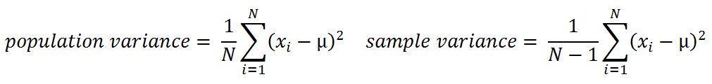
- Variance: This is the mean of squared deviations from the mean (xi = data points, μ = mean of the data, N = number of data points). The dimension of variance is the square of the actual values. The reason to use denominator N-1 for a sample instead of N in the population is due the degree of freedom. 1 degree of freedom lost in a sample by the time of calculating variance is due to extraction of substitution of sample:
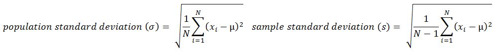
- Standard deviation: This is the square root of variance. By applying the square root on variance, we measure the dispersion with respect to the original variable rather than square of the dimension:
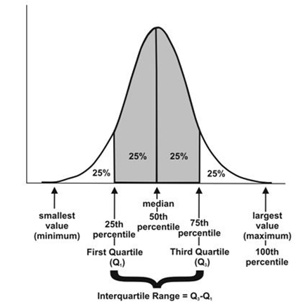
- Quantiles: These are simply identical fragments of the data. Quantiles cover percentiles, deciles, quartiles, and so on. These measures are calculated after arranging the data in ascending order:
- Percentile: This is nothing but the percentage of data points below the value of the original whole data. The median is the 50th percentile, as the number of data points below the median is about 50 percent of the data.
- Decile: This is 10th percentile, which means the number of data points below the decile is 10 percent of the whole data.
- Quartile: This is one-fourth of the data, and also is the 25th percentile. The first quartile is 25 percent of the data, the second quartile is 50 percent of the data, the third quartile is 75 percent of the data. The second quartile is also known as the median or 50th percentile or 5th decile.
- Interquartile range: This is the difference between the third quartile and first quartile. It is effective in identifying outliers in data. The interquartile range describes the middle 50 percent of the data points.
The Python code is as follows:
>>> from statistics import variance, stdev
>>> game_points = np.array([35,56,43,59,63,79,35,41,64,43,93,60,77,24,82])
# Calculate Variance
>>> dt_var = variance(game_points) ; print ("Sample variance:", round(dt_var,2))
# Calculate Standard Deviation
>>> dt_std = stdev(game_points) ; print ("Sample std.dev:", round(dt_std,2))
# Calculate Range
>>> dt_rng = np.max(game_points,axis=0) - np.min(game_points,axis=0) ; print ("Range:",dt_rng)
#Calculate percentiles
>>> print ("Quantiles:")
>>> for val in [20,80,100]:
>>> dt_qntls = np.percentile(game_points,val)
>>> print (str(val)+"%" ,dt_qntls)
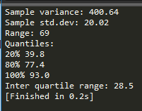
# Calculate IQR
>>> q75, q25 = np.percentile(game_points, [75 ,25]); print ("Inter quartile range:",q75-q25)The output of the preceding code is as follows:
The R code for dispersion (variance, standard deviation, range, quantiles, and IQR) is as follows:
game_points <- c(35,56,43,59,63,79,35,41,64,43,93,60,77,24,82)
dt_var = var(game_points); print(round(dt_var,2))
dt_std = sd(game_points); print(round(dt_std,2))
range_val<-function(x) return(diff(range(x)))
dt_range = range_val(game_points); print(dt_range)
dt_quantile = quantile(game_points,probs = c(0.2,0.8,1.0)); print(dt_quantile)
dt_iqr = IQR(game_points); print(dt_iqr)
- Hypothesis testing: This is the process of making inferences about the overall population by conducting some statistical tests on a sample. Null and alternate hypotheses are ways to validate whether an assumption is statistically significant or not.
- P-value: The probability of obtaining a test statistic result is at least as extreme as the one that was actually observed, assuming that the null hypothesis is true (usually in modeling, against each independent variable, a p-value less than 0.05 is considered significant and greater than 0.05 is considered insignificant; nonetheless, these values and definitions may change with respect to context).
The steps involved in hypothesis testing are as follows:
- Assume a null hypothesis (usually no difference, no significance, and so on; a null hypothesis always tries to assume that there is no anomaly pattern and is always homogeneous, and so on).
- Collect the sample.
- Calculate test statistics from the sample in order to verify whether the hypothesis is statistically significant or not.
- Decide either to accept or reject the null hypothesis based on the test statistic.
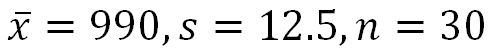
- Example of hypothesis testing: A chocolate manufacturer who is also your friend claims that all chocolates produced from his factory weigh at least 1,000 g and you have got a funny feeling that it might not be true; you both collected a sample of 30 chocolates and found that the average chocolate weight as 990 g with sample standard deviation as 12.5 g. Given the 0.05 significance level, can we reject the claim made by your friend?
The null hypothesis is that μ0 ≥ 1000 (all chocolates weigh more than 1,000 g).
Collected sample:
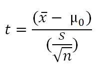
Calculate test statistic:
t = (990 - 1000) / (12.5/sqrt(30)) = - 4.3818
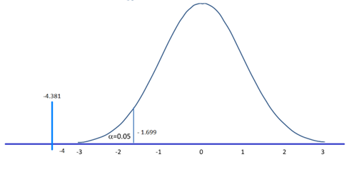
Critical t value from t tables = t0.05, 30 = 1.699 => - t0.05, 30 = -1.699
P-value = 7.03 e-05
Test statistic is -4.3818, which is less than the critical value of -1.699. Hence, we can reject the null hypothesis (your friend's claim) that the mean weight of a chocolate is above 1,000 g.
Also, another way of deciding the claim is by using the p-value. A p-value less than 0.05 means both claimed values and distribution mean values are significantly different, hence we can reject the null hypothesis:
The Python code is as follows:
>>> from scipy import stats
>>> xbar = 990; mu0 = 1000; s = 12.5; n = 30
# Test Statistic
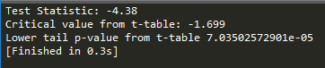
>>> t_smple = (xbar-mu0)/(s/np.sqrt(float(n))); print ("Test Statistic:",round(t_smple,2))
# Critical value from t-table
>>> alpha = 0.05
>>> t_alpha = stats.t.ppf(alpha,n-1); print ("Critical value from t-table:",round(t_alpha,3))
#Lower tail p-value from t-table
>>> p_val = stats.t.sf(np.abs(t_smple), n-1); print ("Lower tail p-value from t-table", p_val) The R code for T-distribution is as follows:
xbar = 990; mu0 = 1000; s = 12.5 ; n = 30
t_smple = (xbar - mu0)/(s/sqrt(n));print (round(t_smple,2))

alpha = 0.05
t_alpha = qt(alpha,df= n-1);print (round(t_alpha,3))

p_val = pt(t_smple,df = n-1);print (p_val)
- Type I and II error: Hypothesis testing is usually done on the samples rather than the entire population, due to the practical constraints of available resources to collect all the available data. However, performing inferences about the population from samples comes with its own costs, such as rejecting good results or accepting false results, not to mention separately, when increases in sample size lead to minimizing type I and II errors:
- Type I error: Rejecting a null hypothesis when it is true
- Type II error: Accepting a null hypothesis when it is false
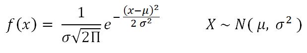
- Normal distribution: This is very important in statistics because of the central limit theorem, which states that the population of all possible samples of size n from a population with mean μ and variance σ2 approaches a normal distribution:
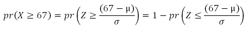
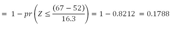
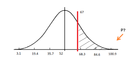
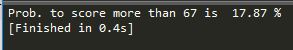
Example: Assume that the test scores of an entrance exam fit a normal distribution. Furthermore, the mean test score is 52 and the standard deviation is 16.3. What is the percentage of students scoring 67 or more in the exam?
The Python code is as follows:
>>> from scipy import stats
>>> xbar = 67; mu0 = 52; s = 16.3

# Calculating z-score
>>> z = (67-52)/16.3

# Calculating probability under the curve
>>> p_val = 1- stats.norm.cdf(z)
>>> print ("Prob. to score more than 67 is ",round(p_val*100,2),"%")
The R code for normal distribution is as follows:
xbar = 67; mu0 = 52; s = 16.3
pr = 1- pnorm(67, mean=52, sd=16.3)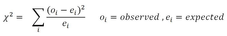
print(paste("Prob. to score more than 67 is ",round(pr*100,2),"%"))- Chi-square: This test of independence is one of the most basic and common hypothesis tests in the statistical analysis of categorical data. Given two categorical random variables X and Y, the chi-square test of independence determines whether or not there exists a statistical dependence between them.
The test is usually performed by calculating χ2 from the data and χ2 with (m-1, n-1) degrees from the table. A decision is made as to whether both variables are independent based on the actual value and table value, whichever is higher:
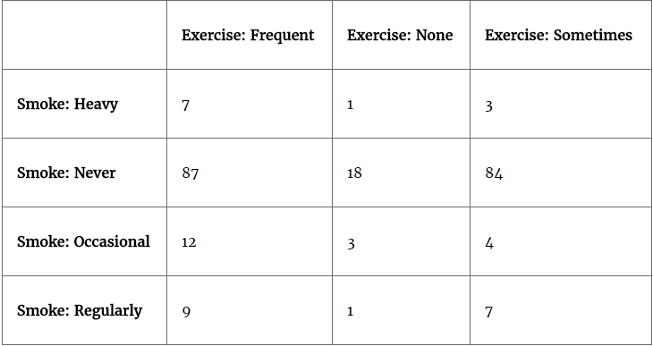
Example: In the following table, calculate whether the smoking habit has an impact on exercise behavior:
The Python code is as follows:
>>> import pandas as pd
>>> from scipy import stats

>>> survey = pd.read_csv("survey.csv")

# Tabulating 2 variables with row & column variables respectively
>>> survey_tab = pd.crosstab(survey.Smoke, survey.Exer, margins = True)
While creating a table using the crosstab function, we will obtain both row and column totals fields extra. However, in order to create the observed table, we need to extract the variables part and ignore the totals:
# Creating observed table for analysis
>>> observed = survey_tab.ix[0:4,0:3]
The chi2_contingency function in the stats package uses the observed table and subsequently calculates its expected table, followed by calculating the p-value in order to check whether two variables are dependent or not. If p-value < 0.05, there is a strong dependency between two variables, whereas if p-value > 0.05, there is no dependency between the variables:
>>> contg = stats.chi2_contingency(observed= observed)
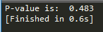
>>> p_value = round(contg[1],3)
>>> print ("P-value is: ",p_value)The p-value is 0.483, which means there is no dependency between the smoking habit and exercise behavior.
The R code for chi-square is as follows:
survey = read.csv("survey.csv",header=TRUE)
tbl = table(survey$Smoke,survey$Exer)
p_val = chisq.test(tbl)- ANOVA: Analyzing variance tests the hypothesis that the means of two or more populations are equal. ANOVAs assess the importance of one or more factors by comparing the response variable means at the different factor levels. The null hypothesis states that all population means are equal while the alternative hypothesis states that at least one is different.
Example: A fertilizer company developed three new types of universal fertilizers after research that can be utilized to grow any type of crop. In order to find out whether all three have a similar crop yield, they randomly chose six crop types in the study. In accordance with the randomized block design, each crop type will be tested with all three types of fertilizer separately. The following table represents the yield in g/m2. At the 0.05 level of significance, test whether the mean yields for the three new types of fertilizers are all equal:
The Python code is as follows:
>>> import pandas as pd
>>> from scipy import stats
>>> fetilizers = pd.read_csv("fetilizers.csv")
Calculating one-way ANOVA using the stats package:
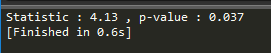
>>> one_way_anova = stats.f_oneway(fetilizers["fertilizer1"], fetilizers["fertilizer2"], fetilizers["fertilizer3"])

>>> print ("Statistic :", round(one_way_anova[0],2),", p-value :",round(one_way_anova[1],3))
Result: The p-value did come as less than 0.05, hence we can reject the null hypothesis that the mean crop yields of the fertilizers are equal. Fertilizers make a significant difference to crops.
The R code for ANOVA is as follows:
fetilizers = read.csv("fetilizers.csv",header=TRUE)
r = c(t(as.matrix(fetilizers)))
f = c("fertilizer1","fertilizer2","fertilizer3")
k = 3; n = 6
tm = gl(k,1,n*k,factor(f))
blk = gl(n,k,k*n)
av = aov(r ~ tm + blk)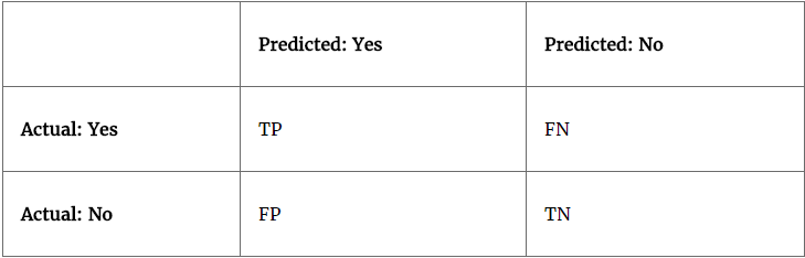
smry = summary(av)- Confusion matrix: This is the matrix of the actual versus the predicted. This concept is better explained with the example of cancer prediction using the model:
Some terms used in a confusion matrix are:
- True positives (TPs): True positives are cases when we predict the disease as yes when the patient actually does have the disease.
- True negatives (TNs): Cases when we predict the disease as no when the patient actually does not have the disease.
- False positives (FPs): When we predict the disease as yes when the patient actually does not have the disease. FPs are also considered to be type I errors.
- False negatives (FNs): When we predict the disease as no when the patient actually does have the disease. FNs are also considered to be type II errors.
- Precision (P): When yes is predicted, how often is it correct?
(TP/TP+FP)
- Recall (R)/sensitivity/true positive rate: Among the actual yeses, what fraction was predicted as yes?
(TP/TP+FN)
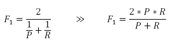
- F1 score (F1): This is the harmonic mean of the precision and recall. Multiplying the constant of 2 scales the score to 1 when both precision and recall are 1:
- Specificity: Among the actual nos, what fraction was predicted as no? Also equivalent to 1- false positive rate:
(TN/TN+FP)
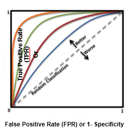
- Area under curve (ROC): Receiver operating characteristic curve is used to plot between true positive rate (TPR) and false positive rate (FPR), also known as a sensitivity and 1- specificity graph:
Area under curve is utilized for setting the threshold of cut-off probability to classify the predicted probability into various classes; we will be covering how this method works in upcoming chapters.
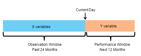
- Observation and performance window: In statistical modeling, the model tries to predict the event in advance rather than at the moment, so that some buffer time will exist to work on corrective actions. For example, a question from a credit card company would be, for example, what is the probability that a particular customer will default in the coming 12-month period? So that I can call him and offer any discounts or develop my collection strategies accordingly.
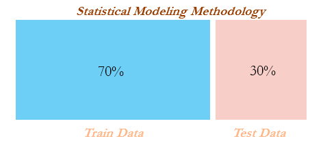
In order to answer this question, a probability of default model (or behavioral scorecard in technical terms) needs to be developed by using independent variables from the past 24 months and a dependent variable from the next 12 months. After preparing data with X and Y variables, it will be split into 70 percent - 30 percent as train and test data randomly; this method is called in-time validation as both train and test samples are from the same time period:
- In-time and out-of-time validation: In-time validation implies obtaining both a training and testing dataset from the same period of time, whereas out-of-time validation implies training and testing datasets drawn from different time periods. Usually, the model performs worse in out-of-time validation rather than in-time due to the obvious reason that the characteristics of the train and test datasets might differ.
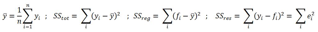
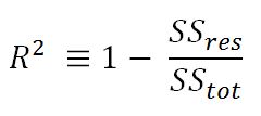
- R-squared (coefficient of determination): This is the measure of the percentage of the response variable variation that is explained by a model. It also a measure of how well the model minimizes error compared with just utilizing the mean as an estimate. In some extreme cases, R-squared can have a value less than zero also, which means the predicted values from the model perform worse than just taking the simple mean as a prediction for all the observations. We will study this parameter in detail in upcoming chapters:
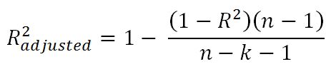
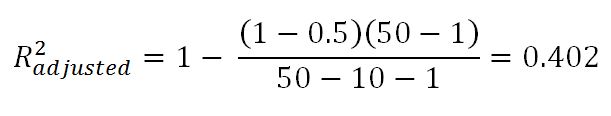
- Adjusted R-squared: The explanation of the adjusted R-squared statistic is almost the same as R-squared but it penalizes the R-squared value if extra variables without a strong correlation are included in the model:
Here, R2 = sample R-squared value, n = sample size, k = number of predictors (or) variables.
Adjusted R-squared value is the key metric in evaluating the quality of linear regressions. Any linear regression model having the value of R2 adjusted >= 0.7 is considered as a good enough model to implement.
Example: The R-squared value of a sample is 0.5, with a sample size of 50 and the independent variables are 10 in number. Calculated adjusted R-squared:
- Maximum likelihood estimate (MLE): This is estimating the parameter values of a statistical model (logistic regression, to be precise) by finding the parameter values that maximize the likelihood of making the observations. We will cover this method in more depth in Chapter 3, Logistic Regression Versus Random Forest.
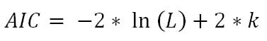
- Akaike information criteria (AIC): This is used in logistic regression, which is similar to the principle of adjusted R-square for linear regression. It measures the relative quality of a model for a given set of data:
Here, k = number of predictors or variables
The idea of AIC is to penalize the objective function if extra variables without strong predictive abilities are included in the model. This is a kind of regularization in logistic regression.
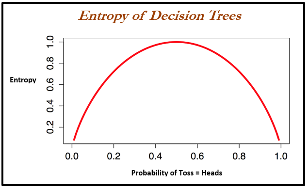
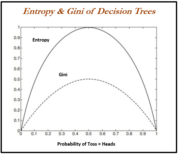
- Entropy: This comes from information theory and is the measure of impurity in the data. If the sample is completely homogeneous, the entropy is zero and if the sample is equally divided, it has an entropy of 1. In decision trees, the predictor with the most heterogeneousness will be considered nearest to the root node to classify given data into classes in a greedy mode. We will cover this topic in more depth in Chapter 4, Tree-Based Machine Learning Models:
Here, n = number of classes. Entropy is maximal at the middle, with the value of 1 and minimal at the extremes as 0. A low value of entropy is desirable as it will segregate classes better:
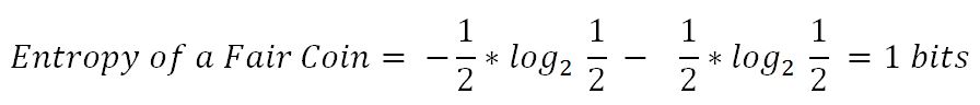
Example: Given two types of coin in which the first one is a fair one (1/2 head and 1/2 tail probabilities) and the other is a biased one (1/3 head and 2/3 tail probabilities), calculate the entropy for both and justify which one is better with respect to modeling:
From both values, the decision tree algorithm chooses the biased coin rather than the fair coin as an observation splitter due to the fact the value of entropy is less.
- Information gain: This is the expected reduction in entropy caused by partitioning the examples according to a given attribute. The idea is to start with mixed classes and to keep partitioning until each node reaches its observations of the purest class. At every stage, the variable with maximum information gain is chosen in greedy fashion:
Information gain = Entropy of parent - sum (weighted % * Entropy of child)
Weighted % = Number of observations in particular child / sum (observations in all child nodes)
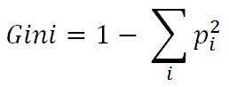
- Gini: Gini impurity is a measure of misclassification, which applies in a multiclass classifier context. Gini works almost the same as entropy, except Gini is faster to calculate:
Here, i = number of classes. The similarity between Gini and entropy is shown as follows:
 Argentina
 Australia
 Austria
 Belgium
 Brazil
 Bulgaria
 Canada
 Chile
Chile
 Colombia
 Cyprus
 Czechia
 Denmark
 Ecuador
 Egypt
Egypt
 Estonia
 Finland
 France
 Germany
 Great Britain
 Greece
 Hungary
 India
India
 Indonesia
 Ireland
 Italy
Italy
 Japan
Japan
 Latvia
 Lithuania
 Luxembourg
 Malaysia
 Malta
Malta
 Mexico
 Netherlands
 New Zealand
 Norway
 Philippines
 Poland
 Portugal
 Romania
 Russia
 Singapore
 Slovakia
 Slovenia
 South Africa
 South Korea
 Spain
Spain
 Sweden
 Switzerland
 Taiwan
 Thailand
 Turkey
 Ukraine
 United States