Packt+ | Advance your knowledge in tech

You're reading from Statistics for Machine Learning

Product typeBook

Published inJul 2017

Reading LevelIntermediate

PublisherPackt

ISBN-139781788295758

Edition1st Edition

Languages

Python

Concepts

Statistics

Author (1)

Pratap Dangeti

Chapter 4. Tree-Based Machine Learning Models

he goal of tree-based methods is to segment the feature space into a number of simple rectangular regions, to subsequently make a prediction for a given observation based on either mean or mode (mean for regression and mode for classification, to be precise) of the training observations in the region to which it belongs. Unlike most other classifiers, models produced by decision trees are easy to interpret. In this chapter, we will be covering the following decision tree-based models on HR data examples for predicting whether a given employee will leave the organization in the near future or not. In this chapter, we will learn the following topics:

Decision trees - simple model and model with class weight tuning
Bagging (bootstrap aggregation)
Random Ffrest - basic random forest and application of grid search on hypyerparameter tuning
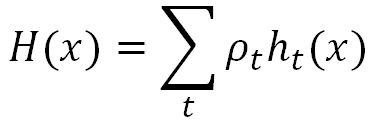
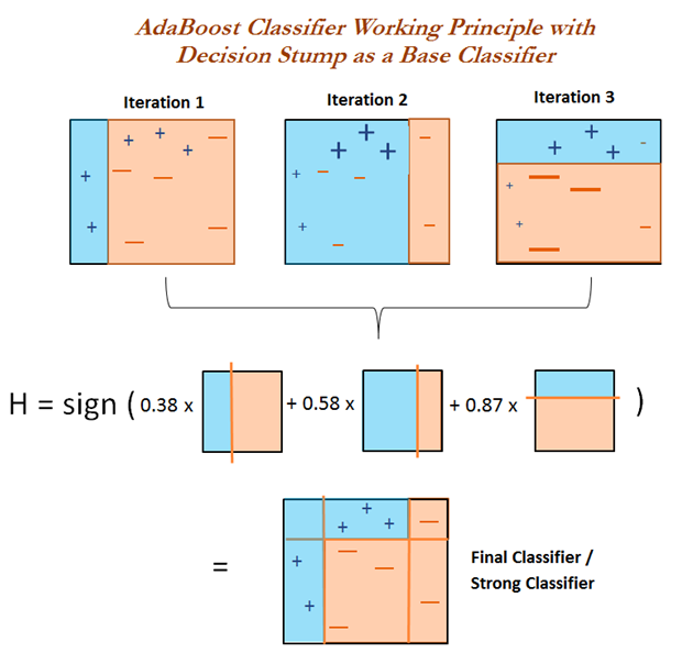
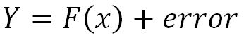
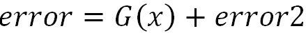
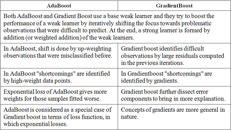
Boosting (AdaBoost, gradient boost, extreme gradient boost - XGBoost)
Ensemble of ensembles (with heterogeneous and...

Introducing decision tree classifiers

Decision tree classifiers produce rules in simple English sentences, which can easily be interpreted and presented to senior management without any editing. Decision trees can be applied to either classification or regression problems. Based on features in data, decision tree models learn a series of questions to infer the class labels of samples.

In the following figure, simple recursive decision rules have been asked by a programmer himself to do relevant actions. The actions would be based on the provided answers for each question, whether yes or no.

Terminology used in decision trees

Decision Trees do not have much machinery as compared with logistic regression. Here we have a few metrics to study. We will majorly focus on impurity measures; decision trees split variables recursively based on set impurity criteria until they reach some stopping criteria (minimum observations per terminal node, minimum observations for split at any node, and so on):

Entropy...

Comparison between logistic regression and decision trees

Before we dive into the coding details of decision trees, here, we will quickly compare the differences between logistic regression and decision trees, so that we will know which model is better and in what way.

Comparison of error components across various styles of models

Errors need to be evaluated in order to measure the effectiveness of the model in order to improve the model's performance further by tuning various knobs. Error components consist of a bias component, variance component, and pure white noise:

Out of the following three regions:

The first region has high bias and low variance error components. In this region, models are very robust in nature, such as linear regression or logistic regression.
Whereas the third region has high variance and low bias error components, in this region models are very wiggly and vary greatly in nature, similar to decision trees, but due to the great amount of variability in the nature of their shape, these models tend to overfit on training data and produce less accuracy on test data.
Last but not least, the middle region, also called the second region, is the ideal sweet spot, in which both bias and variance components are moderate, causing it to create...

Remedial actions to push the model towards the ideal region

Models with either high bias or high variance error components do not produce the ideal fit. Hence, some makeovers are required to do so. In the following diagram, the various methods applied are shown in detail. In the case of linear regression, there would be a high bias component, meaning the model is not flexible enough to fit some non-linearities in data. One turnaround is to break the single line into small linear pieces and fit them into the region by constraining them at knots, also called Linear Spline. Whereas decision trees have a high variance problem, meaning even a slight change in X values leads to large changes in its corresponding Y values, this issue can be resolved by performing an ensemble of the decision trees:

In practice, implementing splines would be a difficult and not so popular method, due to the involvement of the many equations a practitioner has to keep tabs on, in addition to checking the linearity...

HR attrition data example

In this section, we will be using IBM Watson's HR Attrition data (the data has been utilized in the book after taking prior permission from the data administrator) shared in Kaggle datasets under open source license agreement https://www.kaggle.com/pavansubhasht/ibm-hr-analytics-attrition-dataset to predict whether employees would attrite or not based on independent explanatory variables:

>>> import pandas as pd 
>>> hrattr_data = pd.read_csv("WA_Fn-UseC_-HR-Employee-Attrition.csv") 
 
>>> print (hrattr_data.head())

There are about 1470 observations and 35 variables in this data, the top five rows are shown here for a quick glance of the variables:

The following code is used to convert Yes or No categories into 1 and 0 for modeling purposes, as scikit-learn does not fit the model on character/categorical variables directly, hence dummy coding is required to be performed for utilizing the variables in models:

>>> hrattr_data['Attrition_ind...

Decision tree classifier

The DecisionTtreeClassifier from scikit-learn has been utilized for modeling purposes, which is available in the tree submodule:

# Decision Tree Classifier 
>>> from sklearn.tree import DecisionTreeClassifier

The parameters selected for the DT classifier are in the following code with splitting criterion as Gini, Maximum depth as 5, minimum number of observations required for qualifying split is 2, and the minimum samples that should be present in the terminal node is 1:

 >>> dt_fit = DecisionTreeClassifier(criterion="gini", max_depth=5,min_samples_split=2,  min_samples_leaf=1,random_state=42) 
>>> dt_fit.fit(x_train,y_train) 
 
>>> print ("\nDecision Tree - Train Confusion  Matrix\n\n", pd.crosstab(y_train, dt_fit.predict(x_train),rownames = ["Actuall"],colnames = ["Predicted"]))    
>>> from sklearn.metrics import accuracy_score, classification_report    
>>> print ("\nDecision Tree - Train accuracy\n\n",round...

Tuning class weights in decision tree classifier

In the following code, class weights are tuned to see the performance change in decision trees with the same parameters. A dummy DataFrame is created to save all the results of various precision-recall details of combinations:

>>> dummyarray = np.empty((6,10))
>>> dt_wttune = pd.DataFrame(dummyarray)

Metrics to be considered for capture are weight for zero and one category (for example, if the weight for zero category given is 0.2, then automatically, weight for the one should be 0.8, as total weight should be equal to 1), training and testing accuracy, precision for zero category, one category, and overall. Similarly, recall for zero category, one category, and overall are also calculated:

>>> dt_wttune.columns = ["zero_wght","one_wght","tr_accuracy", "tst_accuracy", "prec_zero","prec_one", "prec_ovll", "recl_zero","recl_one","recl_ovll"]

Weights for the zero category are verified from 0.01 to 0.5, as we know we do...

Bagging classifier

As we have discussed already, decision trees suffer from high variance, which means if we split the training data into two random parts separately and fit two decision trees for each sample, the rules obtained would be very different. Whereas low variance and high bias models, such as linear or logistic regression, will produce similar results across both samples. Bagging refers to bootstrap aggregation (repeated sampling with replacement and perform aggregation of results to be precise), which is a general purpose methodology to reduce the variance of models. In this case, they are decision trees.

Aggregation reduces the variance, for example, when we have n independent observations x₁, x₂,..., x_n each with variance σ² and the variance of the mean x̅ of the observations is given by σ²/n, which illustrates by averaging a set of observations that it reduces variance. Here, we are reducing variance by taking many samples from training data (also known as bootstrapping),...

Random forest classifier

Random forests provide an improvement over bagging by doing a small tweak that utilizes de-correlated trees. In bagging, we build a number of decision trees on bootstrapped samples from training data, but the one big drawback with the bagging technique is that it selects all the variables. By doing so, in each decision tree, order of candidate/variable chosen to split remains more or less the same for all the individual trees, which look correlated with each other. Variance reduction on correlated individual entities does not work effectively while aggregating them.

In random forest, during bootstrapping (repeated sampling with replacement), samples were drawn from training data; not just simply the second and third observations randomly selected, similar to bagging, but it also selects the few predictors/columns out of all predictors (m predictors out of total p predictors).

The thumb rule for variable selection of m variables out of total variables p, is m = sqrt...

Random forest classifier - grid search

Tuning parameters in a machine learning model plays a critical role. Here, we are showing a grid search example on how to tune a random forest model:

# Random Forest Classifier - Grid Search 
>>> from sklearn.pipeline import Pipeline 
>>> from sklearn.model_selection import train_test_split,GridSearchCV 
 
>>> pipeline = Pipeline([ ('clf',RandomForestClassifier(criterion='gini',class_weight = {0:0.3,1:0.7}))])

Tuning parameters are similar to random forest parameters apart from verifying all the combinations using the pipeline function. The number of combinations to be evaluated will be (3 x 3 x 2 x 2) *5 =36*5 = 180 combinations. Here 5 is used in the end, due to the cross validation of five-fold:

>>> parameters = { 
...         'clf__n_estimators':(2000,3000,5000), 
...         'clf__max_depth':(5,15,30), 
...         'clf__min_samples_split':(2,3), 
...         'clf__min_samples_leaf':(1,2)  } 

>>> grid_search...

AdaBoost classifier

Boosting is another state-of-the art model that is being used by many data scientists to win so many competitions. In this section, we will be covering the AdaBoost algorithm, followed by gradient boost and extreme gradient boost (XGBoost). Boosting is a general approach that can be applied to many statistical models. However, in this book, we will be discussing the application of boosting in the context of decision trees. In bagging, we have taken multiple samples from the training data and then combined the results of individual trees to create a single predictive model; this method runs in parallel, as each bootstrap sample does not depend on others. Boosting works in a sequential manner and does not involve bootstrap sampling; instead, each tree is fitted on a modified version of an original dataset and finally added up to create a strong classifier:

The preceding figure is the sample methodology on how AdaBoost works. We will cover step-by-step procedures in detail...

Gradient boosting classifier

Gradient boosting is one of the competition-winning algorithms that work on the principle of boosting weak learners iteratively by shifting focus towards problematic observations that were difficult to predict in previous iterations and performing an ensemble of weak learners, typically decision trees. It builds the model in a stage-wise fashion like other boosting methods do, but it generalizes them by allowing optimization of an arbitrary differentiable loss function.

Let's start understanding Gradient Boosting with a simple example, as GB challenges many data scientists in terms of understanding the working principle:

Initially, we fit the model on observations producing 75% accuracy and the remaining unexplained variance is captured in the error term:

Then we will fit another model on the error term to pull the extra explanatory component and add it to the original model, which should improve the overall accuracy:

Now, the model is providing 80% accuracy and...

Comparison between AdaBoosting versus gradient boosting

After understanding both AdaBoost and gradient boost, readers may be curious to see the differences in detail. Here, we are presenting exactly that to quench your thirst!

The gradient boosting classifier from the scikit-learn package has been used for computation here:

# Gradientboost Classifier
>>> from sklearn.ensemble import GradientBoostingClassifier

Parameters used in the gradient boosting algorithms are as follows. Deviance has been used for loss, as the problem we are trying to solve is 0/1 binary classification. The learning rate has been chosen as 0.05, number of trees to build is 5000 trees, minimum sample per leaf/terminal node is 1, and minimum samples needed in a bucket for qualification for splitting is 2:

>>> gbc_fit = GradientBoostingClassifier (loss='deviance', learning_rate=0.05, n_estimators=5000, min_samples_split=2, min_samples_leaf=1, max_depth=1, random_state=42 ) 

>>> gbc_fit.fit(x_train...

Extreme gradient boosting - XGBoost classifier

XGBoost is the new algorithm developed in 2014 by Tianqi Chen based on the Gradient boosting principles. It has created a storm in the data science community since its inception. XGBoost has been developed with both deep consideration in terms of system optimization and principles in machine learning. The goal of the library is to push the extremes of the computation limits of machines to provide scalable, portable, and accurate results:

# Xgboost Classifier
>>> import xgboost as xgb
>>> xgb_fit = xgb.XGBClassifier(max_depth=2, n_estimators=5000, 
learning_rate=0.05)
>>> xgb_fit.fit(x_train, y_train)

>>> print ("\nXGBoost - Train Confusion Matrix\n\n",pd.crosstab(y_train, xgb_fit.predict(x_train),rownames = ["Actuall"],colnames = ["Predicted"]))     
>>> print ("\nXGBoost - Train accuracy",round(accuracy_score(y_train, xgb_fit.predict(x_train)),3))
>>> print ("\nXGBoost  - Train Classification...

Ensemble of ensembles - model stacking

Ensemble of ensembles or model stacking is a method to combine different classifiers into a meta-classifier that has a better generalization performance than each individual classifier in isolation. It is always advisable to take opinions from many people when you are in doubt, when dealing with problems in your personal life too! There are two ways to perform ensembles on models:

Ensemble with different types of classifiers: In this methodology, different types of classifiers (for example, logistic regression, decision trees, random forest, and so on) are fitted on the same training data and results are combined based on either majority voting or average, based on if it is classification or regression problems.
Ensemble with a single type of classifiers, but built separately on various bootstrap samples: In this methodology, bootstrap samples are drawn from training data and, each time, separate models will be fitted (individual models could be decision...

Ensemble of ensembles with different types of classifiers

As briefly mentioned in the preceding section, different classifiers will be applied on the same training data and the results ensembled either taking majority voting or applying another classifier (also known as a meta-classifier) fitted on results obtained from individual classifiers. This means, for meta-classifier X, variables would be model outputs and Y variable would be an actual 0/1 result. By doing this, we will obtain the weightage that should be given for each classifier and those weights will be applied accordingly to classify unseen observations. All three methods of application of ensemble of ensembles are shown here:

Majority voting or average: In this method, a simple mode function (classification problem) is applied to select the category with the major number of appearances out of individual classifiers. Whereas, for regression problems, an average will be calculated to compare against actual values.
Method of application...

Ensemble of ensembles with bootstrap samples using a single type of classifier

In this methodology, bootstrap samples are drawn from training data and, each time, separate models will be fitted (individual models could be decision trees, random forest, and so on) on the drawn sample, and all these results are combined at the end to create an ensemble. This method suits dealing with highly flexible models where variance reduction will still improve performance:

In the following example, AdaBoost is used as a base classifier and the results of individual AdaBoost models are combined using the bagging classifier to generate final outcomes. Nonetheless, each AdaBoost is made up of decision trees with a depth of 1 (decision stumps). Here, we would like to show that classifier inside classifier inside classifier is possible (sounds like the Inception movie though!):

# Ensemble of Ensembles - by applying bagging on simple classifier 
>>> from sklearn.tree import DecisionTreeClassifier 
...

Summary

In this chapter, you have learned the complete details about tree-based models, which are currently the most used in the industry, including individual decision trees with grid search and an ensemble of trees such as bagging, random forest, boosting (including AdaBoost, gradient boost and XGBoost), and finally, ensemble of ensembles, also known as model stacking, for further improving accuracy by reducing variance errors by aggregating results further. In model stacking, you have learned how to determine the weights for each model, so that decisions can be made as to which model to keep in the final results to obtain the best possible accuracy.

In the next chapter, you will be learning k-nearest neighbors and Naive Bayes, which are less computationally intensive than tree-based models. The Naive Bayes model will be explained with an NLP use case. In fact, Naive Bayes and SVM are often used where variables (number of dimensions) are very high in number to classify.

The rest of the chapter is locked

You have been reading a chapter from

Statistics for Machine Learning

Published in: Jul 2017Publisher: PacktISBN-13: 9781788295758

A free Packt account unlocks extra newsletters, articles, discounted offers, and much more. Start advancing your knowledge today.

undefined

Unlock this book and the full library FREE for 7 days

Get unlimited access to 7000+ expert-authored eBooks and videos courses covering every tech area you can think of

Start free trial

Renews at $15.99/month. Cancel anytime

Author (1)

Pratap Dangeti

Pratap Dangeti develops machine learning and deep learning solutions for structured, image, and text data at TCS, analytics and insights, innovation lab in Bangalore. He has acquired a lot of experience in both analytics and data science. He received his master's degree from IIT Bombay in its industrial engineering and operations research program. He is an artificial intelligence enthusiast. When not working, he likes to read about next-gen technologies and innovative methodologies.
Read more about Pratap Dangeti

Other recommended products

Related to this chapter

Machine Learning with scikit-learn Quick Start Guide

Scikit-learn is a robust machine learning library for the Python programming language. It provides a set of supervised and unsupervised learning algorithms. This book is the easiest way to learn how to deploy, optimize and evaluate all the important machine learning algorithms that scikit-learn provides.

BookOct 2018172 pages

Mastering Machine Learning with scikit-learn

This book examines machine learning models including k-nearest neighbors, logistic regression, naive Bayes, random forests, and support vector machines. You will work through document classification, image recognition, and other example problems.

BookJul 2017254 pages

Hands-On Reinforcement Learning with Python

Reinforcement learning is a self-evolving type of machine learning that takes us closer to achieving true artificial intelligence. This easy-to-follow guide explains everything from scratch using rich examples written in Python.

BookJun 2018318 pages

Practical Reinforcement Learning

Reinforcement learning (RL) is becoming a popular tool for constructing autonomous systems that improve themselves with experience. We will break the RL framework into its core building blocks, and provide you with details of each element. This book is divided into three parts. The first part defines Reinforcement Learning and describes the basics and the Python and Java frameworks, which we are going to use later in the book. The second part discusses learning techniques with basic algorithms such as Temporal Difference, Monte Carlo, and Policy Gradient—all with practical examples. Lastly, in the third part we apply Reinforcement Learning with the most recent and widely used algorithms, via practical applications.

BookOct 2017336 pages

Supervised Machine Learning with Python

A supervised learning task infers a function from flagged training data and maps an input to an output based on sample input-output pairs. In this book, you will learn various machine learning techniques (such as linear and logistic regression) and gain the practical knowledge you need to quickly and powerfully apply algorithms to new problems.

BookMay 2019162 pages

Ensemble Machine Learning Cookbook

This book uses a recipe-based approach to showcase the power of machine learning algorithms to build ensemble models using Python libraries. Through this book, you will be able to pick up the code, understand in depth how it works, execute and implement it efficiently. This will be a desk reference to implement a wide range of tasks and solve the common and uncommon problems in ensemble machine learning domain.

BookJan 2019336 pages

Hands-On Ensemble Learning with Python

Ensemble learning can provide the necessary methods to improve the accuracy and performance of existing models. In this book, you'll understand how to combine different machine learning algorithms to produce more accurate results from your models.

BookJul 2019298 pages

Hands-On Reinforcement Learning with R

Reinforcement Learning is an exciting part of machine learning. It has uses in technology from autonomous cars to game playing, and creates algorithms that can adapt to environmental changes. This book helps to understand how to implement RL with R, and explores interesting practical examples, such as using tabular Q-learning to control robots.

BookDec 2019362 pages

Applied Supervised Learning with Python

Applied Supervised Learning with Python provides you a rich understanding of machine learning, one of the most pursued topics in information science, and Python, one of the most popular scripting languages. Through this book, you'll learn Jupyter Notebooks, the technology used in academic and commercial circles with in-line code running support.

BookApr 2019404 pages

Machine Learning with R

Brett Lantz teaches you how to uncover key insights and make new predictions with this hands-on, practical guide to machine learning with R. This third edition is for experienced R users and beginners. The book is fully updated to R 3.6, featuring newer and better libraries, advice on ethical and bias issues, and an introduction to deep learning.

BookApr 2019458 pages

scikit-learn Cookbook

scikit-learn has evolved as a robust library for machine learning applications in python with support for a wide range of supervised and unsupervised learning algorithms. This edition brings to you the various enhancements to its model implementations, API and bug fixes in the latest major release of scikit-learn to support Python. This book covers easy to follow recipes right from mathematical operations to implementing various supervised, unsupervised and deep learning algorithms with scikit-learn. Get practical hands-on knowledge to implement various models and algorithms like Multi-Layer Perceptrons, time-series split, MAE criterion for regression, criteria for gradient boosting, Classifier, Regressor, and much more.

BookNov 2017374 pages

The Supervised Learning Workshop

Taking an engaging and practical approach, The Supervised Learning Workshop teaches you how to predict the output of new data, based on the relationship and behavior of?existing datasets. You’ll learn at your own pace and use Python libraries and Jupyter to build intelligent predictive models.?

BookFeb 2020532 pages

Personalised recommendations for you

Based on your interests and search pattern

Et al.

Ever wonder why speech recognition systems don't understand the Scottish accent, or what would happen if an astronaut only ate mac 'n' cheese, or other spurious reflections you'd have at a bar? We did, then collated those deliberations into absurd research articles with fake figures and methodologies inspired by even more fictionally absurd studies.

BookAug 2023230 pages5

Generative AI with LangChain

This book is a comprehensive introduction to LLMs and LangChain, demystifying the basic mechanics of LangChain, its functionalities, and the myriad of applications it can be integrated into.

BookDec 2023360 pages4

Generative AI with LangChain

This book is a comprehensive introduction to LLMs and LangChain, demystifying the basic mechanics of LangChain, its functionalities, and the myriad of applications it can be integrated into.

BookDec 2023360 pages5

Generative AI with LangChain

This book is a comprehensive introduction to LLMs and LangChain, demystifying the basic mechanics of LangChain, its functionalities, and the myriad of applications it can be integrated into.

BookDec 2023360 pages1

Generative AI with LangChain

This book is a comprehensive introduction to LLMs and LangChain, demystifying the basic mechanics of LangChain, its functionalities, and the myriad of applications it can be integrated into.

BookDec 2023360 pages5

Mastering Tableau 2023

This book is a comprehensive resource to mastering your Tableau skills and becoming a BI expert. As you progress, you will learn how to build advanced dashboards and improve your storytelling to derive key business insight, as well as make you well-versed with advanced functionalities of Tableau in the business intelligence domain.

BookAug 2023684 pages

Building AI Applications with ChatGPT APIs

This guide covers all ChatGPT API features for effortless creation of robust AI powered apps. With its help, you’ll be able to leverage ChatGPT’s cutting-edge NLP models to take your app development skills to the next level. You’ll also work on ten exciting projects that will give you the practical know-how that you can apply to your existing applications.

BookSep 2023258 pages5

Building AI Applications with ChatGPT APIs

This guide covers all ChatGPT API features for effortless creation of robust AI powered apps. With its help, you’ll be able to leverage ChatGPT’s cutting-edge NLP models to take your app development skills to the next level. You’ll also work on ten exciting projects that will give you the practical know-how that you can apply to your existing applications.

BookSep 2023258 pages2

Data Engineering with AWS

Embark on a journey to master data engineering pipelines on AWS! Our book offers a hands-on experience of AWS services for ingesting, transforming, and consuming data. Whether you're an absolute beginner or someone with basic data engineering experience, this guide is an indispensable resource.

BookOct 2023636 pages5

Modern Data Architecture on AWS

Every organization wants an agile, performant, and cost-effective data platform that meets all their current and future business needs. Purpose-built AWS analytics services and their features play a big part in building such a modern data platform. This book brings to you all the design and architectural patterns that’ll help you achieve this goal.

BookAug 2023420 pages5

Practical Guide to Applied Conformal Prediction in Python

Discover the power of Conformal Prediction with the "Practical Guide to Applied Conformal Prediction in Python." Master the latest techniques to quantify uncertainty in machine learning and computer vision models, and seamlessly apply them to your industry applications.

BookDec 2023240 pages

TinyML Cookbook

With over 70 project-based recipes, the TinyML Cookbook is a practical guide that will help you to get the most out of your microcontrollers. It provides a comprehensive understanding of the theoretical foundations while giving you hands-on experience training ML models for deployment on Arduino Nano 33 BLE Sense, Raspberry Pi Pico, and SparkFun RedBoard Artemis Nano microcontrollers.

BookNov 2023664 pages

Logistic regression	Decision trees
Logistic regression model looks like an equation between independent variables with respect to its dependent variable.	Tree classifiers produce rules in simple English sentences, which can be easily explained to senior management.
Logistic regression is a parametric model, in which the model is defined by having parameters multiplied by independent variables to predict the dependent variable.	Decision Trees are a non-parametric model, in which no pre-assumed parameter exists. Implicitly performs variable screening or feature selection.
Assumptions are made on response (or dependent) variable, with binomial or Bernoulli distribution.	No assumptions are made on the underlying distribution of the data...