

Working with Tabular Data in pandas
If NumPy is used on matrix data and linear algebraic operations, pandas is designed to work with data in the form of tables. Just like NumPy, pandas can be installed in your Python environment using the pip package manager:
$ pip install pandas
If you are using Anaconda, you can download it using the following command:
$ conda install pandas
Once the installation process completes, fire off a Python interpreter and try importing the library:
>>> import pandas as pd
If this command runs without any error message, then you have successfully installed pandas. With that, let's move on with our discussions, beginning with the most commonly used data structure in pandas, DataFrame, which can represent table data: two-dimensional data with row and column labels. This is to be contrasted with NumPy arrays, which can take on any dimension but do not support labeling.
Initializing a DataFrame Object
There are multiple ways to initialize a DataFrame object. First, we can manually create one by passing in a Python dictionary, where each key should be the name of a column, and the value for that key should be the data included for that column, in the form of a list or a NumPy array.
For example, in the following code, we are creating a table with two rows and three columns. The first column contains the numbers 1 and 2 in order, the second contains 3 and 4, and the third 5 and 6:
>>> import pandas as pd
>>> my_dict = {'col1': [1, 2], 'col2': np.array([3, 4]),'col3': [5, 6]}
>>> df = pd.DataFrame(my_dict)
>>> df
     col1    col2    col3
0    1       3       5
1    2       4       6
The first thing to note about DataFrame objects is that, as you can see from the preceding code snippet, when one is printed out, the output is automatically formatted by the backend of pandas. The tabular format makes the data represented in that object more readable. Additionally, when a DataFrame object is printed out in a Jupyter notebook, similar formatting is utilized for the same purpose of readability, as illustrated in the following screenshot:
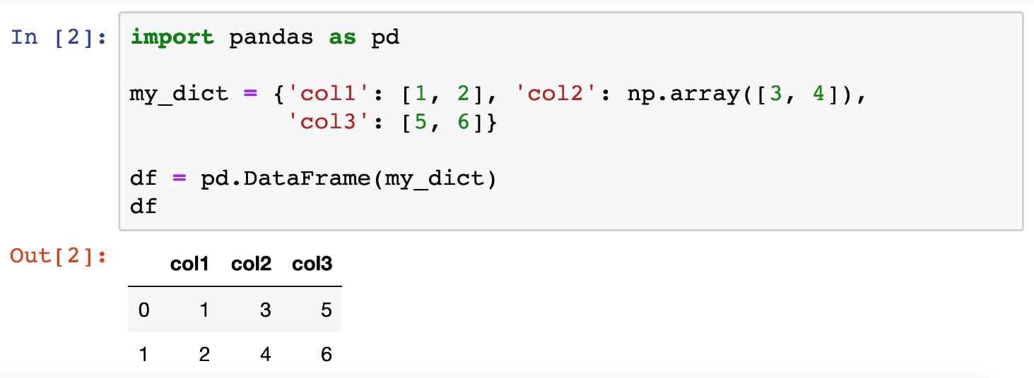
Figure 2.1: Printed DataFrame objects in Jupyter Notebooks
Another common way to initialize a DataFrame object is that when we already have its data represented by a 2D NumPy array, we can directly pass that array to the DataFrame class. For example, we can initialize the same DataFrame we looked at previously with the following code:
>>> my_array = np.array([[1, 3, 5], [2, 4, 6]])
>>> alt_df = pd.DataFrame(my_array, columns=['col1', 'col2', 'col3'])
>>> alt_df
     col1    col2    col3
0    1       3       5
1    2       4       6
That said, the most common way in which a DataFrame object is initialized is through the pd.read_csv() function, which, as the name suggests, reads in a CSV file (or any text file formatted in the same way but with a different separating special character) and renders it as a DataFrame object. We will see this function in action in the next section, where we will understand the working of more functionalities from the pandas library.
Accessing Rows and Columns
Once we already have a table of data represented in a DataFrame object, there are numerous options we can use to interact with and manipulate this table. For example, the first thing we might care about is accessing the data of certain rows and columns. Luckily, pandas offers intuitive Python syntax for this task.
To access a group of rows or columns, we can take advantage of the loc method, which takes in the labels of the rows/columns we are interested in. Syntactically, this method is used with square brackets (to simulate the indexing syntax in Python). For example, using the same table from our previous section, we can pass in the name of a row (for example, 0):
>>> df.loc[0]
col1    1
col2    3
col3    5
Name: 0, dtype: int64
We can see that the object returned previously contains the information we want (the first row, and the numbers 1, 3, and 5), but it is formatted in an unfamiliar way. This is because it is returned as a Series object. Series objects are a special case of DataFrame objects that only contain 1D data. We don't need to pay too much attention to this data structure as its interface is very similar to that of DataFrame.
Still considering the loc method, we can pass in a list of row labels to access multiple rows. The following code returns both rows in our example table:
>>> df.loc[[0, 1]]
     col1    col2    col3
0    1       3       5
1    2       4       6
Say you want to access the data in our table column-wise. The loc method offers that option via the indexing syntax that we are familiar with in NumPy arrays (row indices separated by column indices by a comma). Accessing the data in the first row and the second and third columns:
>>> df.loc[0, ['col2', 'col3']]
col2    3
col3    5
Name: 0, dtype: int64
Note that if you'd like to return a whole column in a DataFrame object, you can use the special character colon, :, in the row index to indicate that all the rows should be returned. For example, to access the 'col3' column in our DataFrame object, we can say df.loc[:, 'col3']. However, in this special case of accessing a whole column, there is another simple syntax: just using the square brackets without the loc method, as follows:
>>> df['col3']
0    5
1    6
Name: col3, dtype: int64
Earlier, we said that when accessing individual rows or columns in a DataFrame, Series objects are returned. These objects can be iterated using, for example, a for loop:
>>> for item in df.loc[:, 'col3']:
...     print(item)
5
6
In terms of changing values in a DataFrame object, we can use the preceding syntax to assign new values to rows and columns:
>>> df.loc[0] = [3, 6, 9]  # change first row
>>> df
     col1    col2    col3
0    3       6       9
1    2       4       6
>>> df['col2'] = [0, 0]  # change second column
>>> df
     col1    col2    col3
0    3       0       9
1    2       0       6
Additionally, we can use the same syntax to declare new rows and columns:
>>> df['col4'] = [10, 10]
>>> df.loc[3] = [1, 2, 3, 4]
>>> df
     col1    col2    col3    col4
0    3       0       9       10
1    2       0       6       10
3    1       2       3       4
Finally, even though it is more common to access rows and columns in a DataFrame object by specifying their actual indices in the loc method, it is also possible to achieve the same effect using an array of Boolean values (True and False) to indicate which items should be returned.
For example, we can access the items in the second row and the second and fourth columns in our current table by writing the following:
>>> df.loc[[False, True, False], [False, True, False, True]]
     col2    col4
1    0       10
Here, the Boolean index list for the rows [False, True, False] indicates that only the second element (that is, the second row) should be returned, while the Boolean index list for the columns, similarly, specifies that the second and fourth columns are to be returned.
While this method of accessing elements in a DataFrame object might seem strange, it is highly valuable for filtering and replacing tasks. Specifically, instead of passing in lists of Boolean values as indices, we can simply use a conditional inside the loc method. For example, to display our current table, just with the columns whose values in their first row are larger than 5 (which should be the third and fourth columns), we can write the following:
>>> df.loc[:, df.loc[0] > 5]
     col3    col4
0    9       10
1    6       10
3    3       4
Again, this syntax is specifically useful in terms of filtering out the rows or columns in a DataFrame object that satisfy some condition and potentially assign new values to them. A special case of this functionality is find-and-replace tasks (which we will go through in the next section).
Manipulating DataFrames
In this section, we will try out a number of methods and functions for DataFrame objects that are used to manipulate the data within those objects. Of course, there are numerous other methods that are available (which you can find in the official documentation: https://pandas.pydata.org/pandas-docs/stable/reference/api/pandas.DataFrame.html). However, the methods given in the following table are among the most commonly used and offer great power and flexibility in terms of helping us to create, maintain, and mutate our data tables:
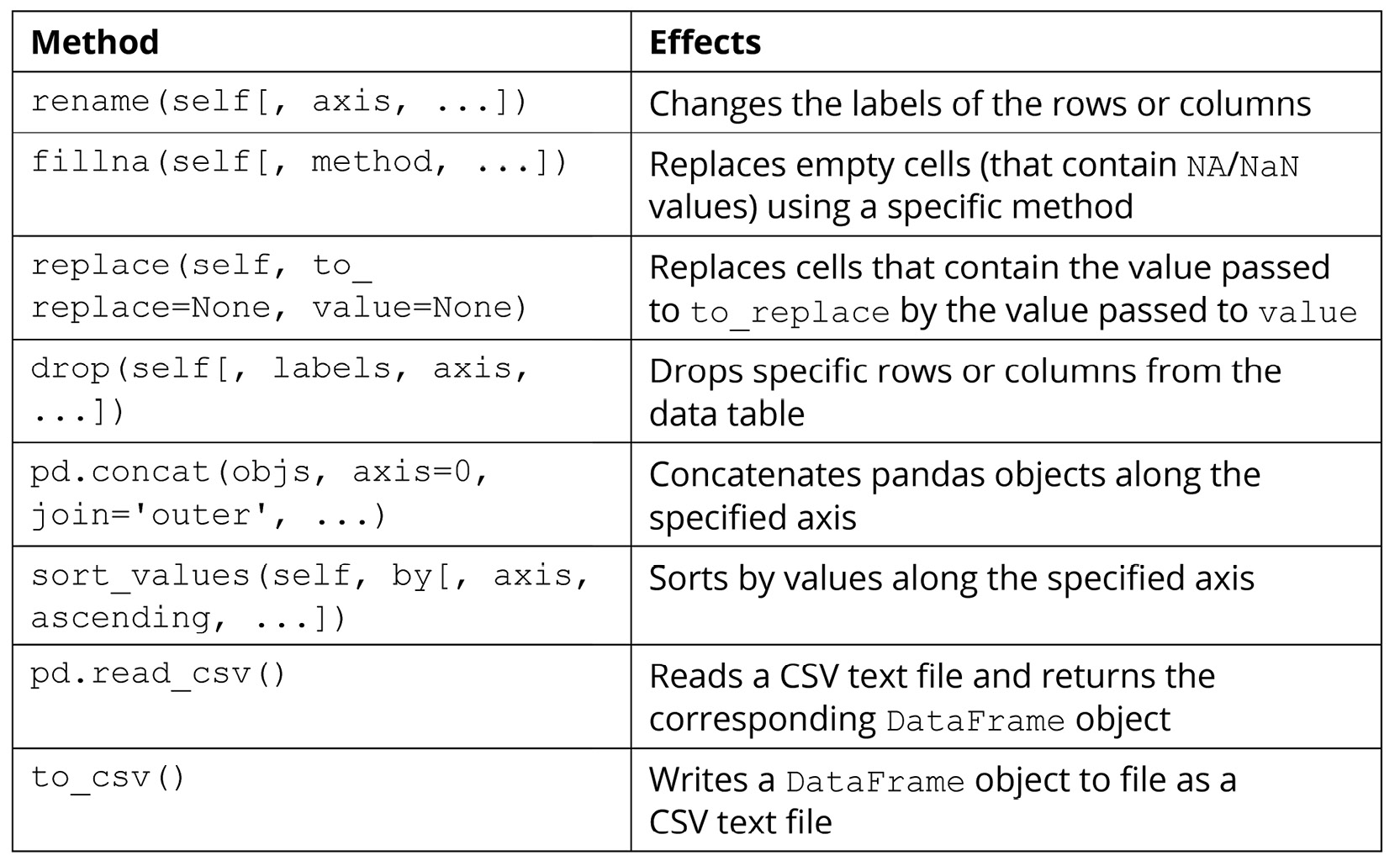
Figure 2.2: Methods used to manipulate pandas data
The following exercise will demonstrate the effects of the preceding methods for better understanding.
Exercise 2.02: Data Table Manipulation
In this hands-on exercise, we will go through the functions and methods included in the preceding section. Our goal is to see the effects of those methods, and to perform common data manipulation techniques such as renaming columns, filling in missing values, sorting values, or writing a data table to file.
Perform the following steps to complete this exercise:
- From the GitHub repository of this workshop, copy the
Exercise2.02/dataset.csvfile within theChapter02folder to a new directory. The content of the file is as follows:id,x,y,z 0,1,1,3 1,1,0,9 2,1,3, 3,2,0,10 4,1,,4 5,2,2,3
- Inside that new directory, create a new Jupyter notebook. Make sure that this notebook and the CSV file are in the same location.
- In the first cell of this notebook, import both pandas and NumPy, and then read in the
dataset.csvfile using thepd.read_csv()function. Specify theindex_colargument of this function to be'id', which is the name of the first column in our sample dataset:import pandas as pd import numpy as np df = pd.read_csv('dataset.csv', index_col='id') - When we print this newly created
DataFrameobject out, we can see that its values correspond directly to our original input file:x y z id 0 1 1.0 3.0 1 1 0.0 9.0 2 1 3.0 NaN 3 2 0.0 10.0 4 1 NaN 4.0 5 2 2.0 3.0
Notice the
NaN(Not a Number) values here;NaNis the default value that will be filled in empty cells of aDataFrameobject upon initialization. Since our original dataset was purposefully designed to contain two empty cells, those cells were appropriately filled in withNaN, as we can see here.Additionally,
NaNvalues are registered as floats in Python, which is why the data type of the two columns containing them are converted into floats accordingly (indicated by the decimal points in the values). - In the next cell, rename the current columns to
'col_x','col_y', and'col_z'with therename()method. Here, thecolumnsargument should be specified with a Python dictionary mapping each old column name to its new name:df = df.rename(columns={'x': 'col_x', 'y': 'col_y', \ 'z': 'col_z'})This change can be observed when
dfis printed out after the line of code is run:col_x col_y col_z id 0 1 1.0 3.0 1 1 0.0 9.0 2 1 3.0 NaN 3 2 0.0 10.0 4 1 NaN 4.0 5 2 2.0 3.0
- In the next cell, use the
fillna()function to replace theNaNvalues with zeros. After this, convert all the data in our table into integers usingastype(int):df = df.fillna(0) df = df.astype(int)
The resulting
DataFrameobject now looks like this:col_x col_y col_z id 0 1 1 3 1 1 0 9 2 1 3 0 3 2 0 10 4 1 0 4 5 2 2 3
- In the next cell, remove the second, fourth, and fifth rows from the dataset by passing the
[1, 3, 4]list to thedropmethod:df = df.drop([1, 3, 4], axis=0)
Note that the
axis=0argument specifies that the labels we are passing to the method specify rows, not columns, of the dataset. Similarly, to drop specific columns, you can use a list of column labels while specifyingaxis=1.The resulting table now looks like this:
     col_x    col_y    col_z
id
0    1        1        3
2    1        3        0
5    2        2        3
- In the next cell, create an all-zero, 2 x 3
DataFrameobject with the corresponding column labels as the currentdfvariable:zero_df = pd.DataFrame(np.zeros((2, 3)), columns=['col_x', 'col_y', \ 'col_z'])
The output is as follows:
     col_x    col_y    col_z
0    0.0      0.0      0.0
1    0.0      0.0      0.0
- In the next code cell, use the
pd.concat()function to concatenate the twoDataFrameobjects together (specifyaxis=0so that the two tables are concatenated vertically, instead of horizontally):df = pd.concat([df, zero_df], axis=0)
Our current
dfvariable now prints out the following (notice the two newly concatenated rows at the bottom of the table):col_x col_y col_z 0 1.0 1.0 3.0 2 1.0 3.0 0.0 5 2.0 2.0 3.0 0 0.0 0.0 0.0 1 0.0 0.0 0.0
- In the next cell, sort our current table in increasing order by the data in the
col_xcolumn:df = df.sort_values('col_x', axis=0)The resulting dataset now looks like this:
     col_x    col_y    col_z
0    0.0      0.0      0.0
1    0.0      0.0      0.0
0    1.0      1.0      3.0
2    1.0      3.0      0.0
5    2.0      2.0      3.0
- Finally, in another code cell, convert our table into the integer data type (the same way as before) and use the
to_csv()method to write this table to a file. Pass in'output.csv'as the name of the output file and specifyindex=Falseso that the row labels are not included in the output:df = df.astype(int) df.to_csv('output.csv', index=False)The written output should look as follows:
col_x, col_y, col_z
0,0,0
0,0,0
1,1,3
1,3,0
2,2,3
And that is the end of this exercise. Overall, this exercise simulated a simplified workflow of working with a tabular dataset: reading in the data, manipulating it in some way, and finally writing it to file.
Note
To access the source code for this specific section, please refer to https://packt.live/38ldQ8O.
You can also run this example online at https://packt.live/3dTzkL6.
In the next and final section on pandas, we will consider a number of more advanced functionalities offered by the library.
Advanced Pandas Functionalities
Accessing and changing the values in the rows and columns of a DataFrame object are among the simplest ways to work with tabular data using the pandas library. In this section, we will go through three other options that are more complicated but also offer powerful options for us to manipulate our DataFrame objects. The first is the apply() method.
If you are already familiar with the concept of this method for other data structures, the same goes for this method, which is implemented for DataFrame objects. In a general sense, this method is used to apply a function to all elements within a DataFrame object. Similar to the concept of vectorization that we discussed earlier, the resulting DataFrame object, after the apply() method, will have its elements as the result of the specified function when each element of the original data is fed to it.
For example, say we have the following DataFrame object:
>>> df = pd.DataFrame({'x': [1, 2, -1], 'y': [-3, 6, 5], \
                       'z': [1, 3, 2]})
>>> df
     x     y     z
0    1     -3    1
1    2     6     3
2    -1    5     2
Now, say we'd like to create another column whose entries are the entries in the x_squared column. We can then use the apply() method, as follows:
>>> df['x_squared'] = df['x'].apply(lambda x: x ** 2)
>>> df
     x     y    z    x_squared
0    1     -3   1    1
1    2     6    3    4
2    -1    5    2    1
The term lambda x: x ** 2 here is simply a quick way to declare a function without a name. From the printed output, we see that the 'x_squared' column was created correctly. Additionally, note that with simple functions such as the square function, we can actually take advantage of the simple syntax of NumPy arrays that we are already familiar with. For example, the following code will have the same effect as the one we just considered:
>>> df['x_squared'] = df['x'] ** 2
However, with a function that is more complex and cannot be vectorized easily, it is better to fully write it out and then pass it to the apply() method. For example, let's say we'd like to create a column, each cell of which should contain the string 'even' if the element in the x column in the same row is even, and the string 'odd' otherwise.
Here, we can create a separate function called parity_str() that takes in a number and returns the corresponding string. This function can then be used with the apply() method on df['x'], as follows:
>>> def parity_str(x):
...     if x % 2 == 0:
...         return 'even'

...     return 'odd'
>>> df['x_parity'] = df['x'].apply(parity_str)
>>> df
     x     y     z    x_squared    x_parity
0    1     -3    1    1            odd
1    2     6     3    4            even
2    -1    5     2    1            odd
Another commonly used functionality in pandas that is slightly more advanced is the pd.get_dummies() function. This function implements the technique called one-hot encoding, which is to be used on a categorical attribute (or column) in a dataset.
We will discuss the concept of categorical attributes, along with other types of data, in more detail in the next chapter. For now, we simply need to keep in mind that plain categorical data sometimes cannot be interpreted by statistical and machine learning models. Instead, we would like to have a way to translate the categorical characteristic of the data into a numerical form while ensuring that no information is lost.
One-hot encoding is one such method; it works by generating a new column/attribute for each unique value and populating the cells in the new column with Boolean data, indicating the values from the original categorical attribute.
This method is easier to understand via examples, so let's consider the new 'x_parity' column we created in the preceding example:
>>> df['x_parity']
0     odd
1    even
2     odd
Name: x_parity, dtype: object
This column is considered a categorical attribute since its values belong to a specific set of categories (in this case, the categories are odd and even). Now, by calling pd.get_dummies() on the column, we obtain the following DataFrame object:
>>> pd.get_dummies(df['x_parity'])
     even    odd
0    0       1
1    1       0
2    0       1
As we can observe from the printed output, the DataFrame object includes two columns that correspond to the unique values in the original categorical data (the 'x_parity' column). For each row, the column that corresponds to the value in the original data is set to 1 and the other column(s) is/are set to 0. For example, the first row originally contained odd in the 'x_parity' column, so its new odd column is set to 1.
We can see that with one-hot encoding, we can convert any categorical attribute into a new set of binary attributes, making the data readably numerical for statistical and machine learning models. However, a big drawback of this method is the increase in dimensionality, as it creates a number of new columns that are equal to the number of unique values in the original categorical attribute. As such, this method can cause our table to greatly increase in size if the categorical data contains many different values. Depending on your computing power and resources, the recommended limit for the number of unique categorical values for the method is 50.
The value_counts() method is another valuable tool in pandas that you should have in your toolkit. This method, to be called on a column of a DataFrame object, returns a list of unique values in that column and their respective counts. This method is thus only applicable to categorical or discrete data, whose values belong to a given, predetermined set of possible values.
For example, still considering the 'x_parity' attribute of our sample dataset, we'll inspect the effect of the value_counts() method:
>>> df['x_parity'].value_counts()
odd     2
even    1
Name: x_parity, dtype: int64
We can see that in the 'x_parity' column, we indeed have two entries (or rows) whose values are odd and one entry for even. Overall, this method is quite useful in determining the distribution of values in, again, categorical and discrete data types.
The next and last advanced functionality of pandas that we will discuss is the groupby operation. This operation allows us to separate a DataFrame object into subgroups, where the rows in a group all share a value in a categorical attribute. From these separate groups, we can then compute descriptive statistics (a concept we will delve into in the next chapter) to explore our dataset further.
We will see this in action in our next exercise, where we'll explore a sample student dataset.
Exercise 2.03: The Student Dataset
By considering a sample of what can be a real-life dataset, we will put our knowledge of pandas' most common functions to use, including what we have been discussing, as well as the new groupby operation.
Perform the following steps to complete this exercise:
- Create a new Jupyter notebook and, in its first cell, run the following code to generate our sample dataset:
import pandas as pd
student_df = pd.DataFrame({'name': ['Alice', 'Bob', 'Carol', \
                                    'Dan', 'Eli', 'Fran'],\
                           'gender': ['female', 'male', \
                                      'female', 'male', \
                                      'male', 'female'],\
                           'class': ['FY', 'SO', 'SR', \
                                     'SO',' JR', 'SR'],\
                           'gpa': [90, 93, 97, 89, 95, 92],\
                           'num_classes': [4, 3, 4, 4, 3, 2]})
student_df
This code will produce the following output, which displays our sample dataset in tabular form:
     name    gender    class    gpa    num_classes
0    Alice   female    FY       90     4
1    Bob     male      SO       93     3
2    Carol   female    SR       97     4
3    Dan     male      SO       89     4
4    Eli     male      JR       95     3
5    Fran    female    SR       92     2
Most of the attributes in our dataset are self-explanatory: in each row (which represents a student),
namecontains the name of the student,genderindicates whether the student is male or female,classis a categorical attribute that can take four unique values (FYfor first-year,SOfor sophomore,JRfor junior, andSRfor senior),gpadenotes the cumulative score of the student, and finally,num_classesholds the information of how many classes the student is currently taking. - In a new code cell, create a new attribute named
'female_flag'whose individual cells should hold the Boolean valueTrueif the corresponding student is female, andFalseotherwise.Here, we can see that we can take advantage of the
apply()method while passing in a lambda object, like so:student_df['female_flag'] = student_df['gender']\ .apply(lambda x: x == 'female')
However, we can also simply declare the new attribute using the
student_df['gender'] == 'female'expression, which evaluates the conditionals sequentially in order:student_df['female_flag'] = student_df['gender'] == 'female'
- This newly created attribute contains all the information included in the old
gendercolumn, so we will remove the latter from our dataset using thedrop()method (note that we need to specify theaxis=1argument since we are dropping a column):student_df = student_df.drop('gender', axis=1)Our current
DataFrameobject should look as follows:name class gpa num_classes female_flag 0 Alice FY 90 4 True 1 Bob SO 93 3 False 2 Carol SR 97 4 True 3 Dan SO 89 4 False 4 Eli JR 95 3 False 5 Fran SR 92 2 True
- In a new code cell, write an expression to apply one-hot encoding to the categorical attribute,
class:pd.get_dummies(student_df['class'])
- In the same code cell, take this expression and include it in a
pd.concat()function to concatenate this newly createdDataFrameobject to our old one, while simultaneously dropping theclasscolumn (as we now have an alternative for the information in this attribute):student_df = pd.concat([student_df.drop('class', axis=1), \ pd.get_dummies(student_df['class'])], axis=1)The current dataset should now look as follows:
     name    gpa    num_classes    female_flag    JR    FY    SO    SR
0    Alice   90     4              True           1     0     0     0
1    Bob     93     3              False          0     0     1     0
2    Carol   97     4              True           0     0     0     1
3    Dan     89     4              False          0     0     1     0
4    Eli     95     3              False          0     1     0     0
5    Fran    92     2              True           0     0     0     1
- In the next cell, call the
groupby()method onstudent_dfwith thefemale_flagargument and assign the returned value to a variable namedgender_group:gender_group = student_df.groupby('female_flag')As you might have guessed, here, we are grouping the students of the same gender into groups, so male students will be grouped together, and female students will also be grouped together but separate from the first group.
It is important to note that when we attempt to print out this
GroupByobject stored in thegender_groupvariable, we only obtain a generic, memory-based string representation:<pandas.core.groupby.generic.DataFrameGroupBy object at 0x11d492550>
- Now, we'd like to compute the average GPA of each group in the preceding grouping. To do that, we can use the following simple syntax:
gender_group['gpa'].mean()
The output will be as follows:
female_flag
False    92.333333
True     93.000000
Name: gpa, dtype: float64
Our command on the
gender_groupvariable is quite intuitive: we'd like to compute the average of a specific attribute, so we access that attribute using square brackets,[' gpa '], and then call themean()method on it. - Similarly, we can compute the total number of classes taking male students, as well as that number for the female students, with the following code:
gender_group['num_classes'].sum()
The output is as follows:
female_flag
False    10
True     10
Name: num_classes, dtype: int64
Throughout this exercise, we have reminded ourselves of some of the important methods available in pandas, and seen the effects of the groupby operation in action via a sample real-life dataset. This exercise also concludes our discussion on the pandas library, the premier tool for working with tabular data in Python.
Note
To access the source code for this specific section, please refer to https://packt.live/2NOe5jt.
You can also run this example online at https://packt.live/3io2gP2.
In the final section of this chapter, we will talk about the final piece of a typical data science/scientific computing pipeline: data visualization.