Implementing neural network-based RL policies for continuous action spaces and continuous-control problems

Reinforcement learning has been used to achieve the state of the art in many control problems, not only in games as varied as Atari, Go, Chess, Shogi, and StarCraft, but also in real-world deployments, such as HVAC control systems.

In environments where the action space is continuous, meaning that the actions are real-valued, a real-valued, continuous policy distribution is necessary. A continuous probability distribution can be used to represent an RL agent's policy when the action space of the environment contains real numbers. In a general sense, such distributions can be used to describe the possible results of a random variable when the random variable can take any (real) value.

Once the recipe is complete, you will have a complete script to control a car in two dimensions to drive up a hill using the MountainCarContinuous environment with a continuous action space. A screenshot from the MountainCarContinuous environment is shown here:

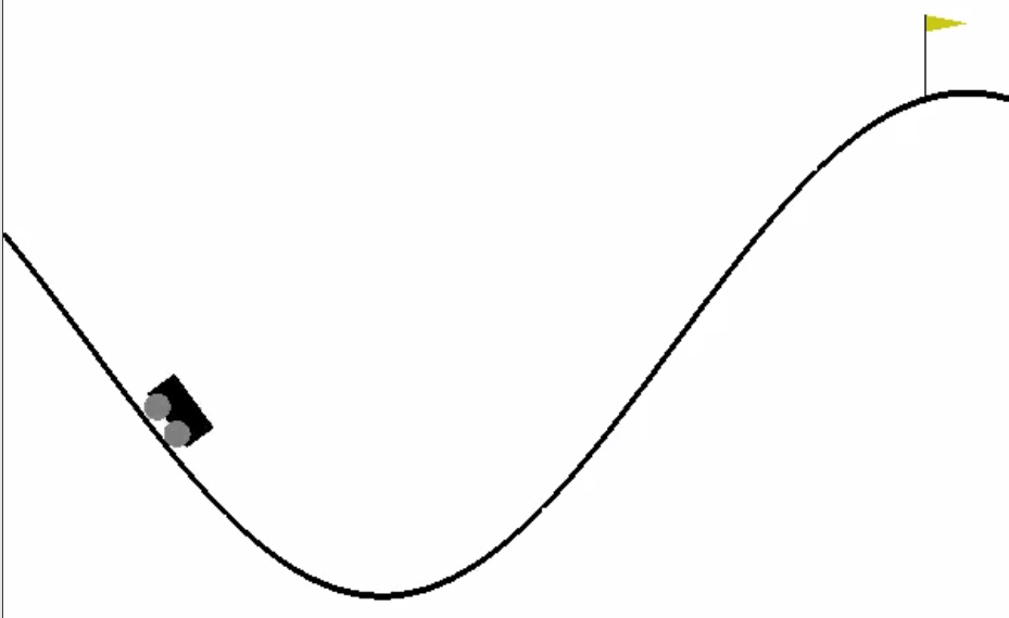
Figure 1.5 – A screenshot of the MountainCarContinuous environment

Getting ready

Activate the tf2rl-cookbook Conda Python environment and run the following command to install and import the necessary Python packages for this recipe:

pip install --upgrade tensorflow_probability
import tensorflow_probability as tfp
import seaborn as sns

Let's get started.

How to do it…

We will begin by creating continuous policy distributions using TensorFlow 2.x and the tensorflow_probability library and build upon the necessary action sampling methods to generate action for a given continuous space of an RL environment:

1. We create a continuous policy distribution in TensorFlow 2.x using the tensorflow_probability library. We will use a Gaussian/normal distribution to create a policy distribution over continuous values:

   sample_actions = continuous_policy.sample(500)
   sns.distplot(sample_actions)

2. Next, we visualize a continuous policy distribution:

   sample_actions = continuous_policy.sample(500)
   sns.distplot(sample_actions)

   The preceding code will generate a distribution plot of the continuous policy, like the plot shown here:

   

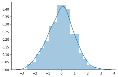
   Figure 1.6 – A distribution plot of the continuous policy

3. Let's now implement a continuous policy distribution using a Gaussian/normal distribution:

   mu = 0.0  # Mean = 0.0
   sigma = 1.0  # Std deviation = 1.0
   continuous_policy = tfp.distributions.Normal(loc=mu,
                                                scale=sigma)
   # action = continuous_policy.sample(10)
   for i in range(10):
       action = continuous_policy.sample(1)
       print(action)

   The preceding code should print something similar to what is shown in the following code block:

   tf.Tensor([-0.2527136], shape=(1,), dtype=float32)
   tf.Tensor([1.3262751], shape=(1,), dtype=float32)
   tf.Tensor([0.81889665], shape=(1,), dtype=float32)
   tf.Tensor([1.754675], shape=(1,), dtype=float32)
   tf.Tensor([0.30025303], shape=(1,), dtype=float32)
   tf.Tensor([-0.61728036], shape=(1,), dtype=float32)
   tf.Tensor([0.40142158], shape=(1,), dtype=float32)
   tf.Tensor([1.3219402], shape=(1,), dtype=float32)
   tf.Tensor([0.8791297], shape=(1,), dtype=float32)
   tf.Tensor([0.30356944], shape=(1,), dtype=float32)

   Important note

   The values of the action that you get will differ from what is shown here because they will be sampled from the Gaussian distribution, which is not a deterministic process.

4. Let's now move one step further and implement a multi-dimensional continuous policy. A multivariate Gaussian distribution can be used to represent multi-dimensional continuous policies. Such polices are useful for agents when acting in environments with action spaces that are multi-dimensional, as well as continuous and real-valued:

   mu = [0.0, 0.0]
   covariance_diag = [3.0, 3.0]
   continuous_multidim_policy = tfp.distributions.MultivariateNormalDiag(loc=mu, scale_diag=covariance_diag)
   # action = continuous_multidim_policy.sample(10)
   for i in range(10):
       action = continuous_multidim_policy.sample(1)
       print(action)

   The preceding code should print something similar to what follows:

   Important note

   The values of the action that you get will differ from what is shown here because they will be sampled from the multivariate Gaussian/normal distribution, which is not a deterministic process).

    tf.Tensor([[ 1.7003113 -2.5801306]], shape=(1, 2), dtype=float32)
   tf.Tensor([[ 2.744986  -0.5607129]], shape=(1, 2), dtype=float32)
   tf.Tensor([[ 6.696332  -3.3528223]], shape=(1, 2), dtype=float32)
   tf.Tensor([[ 1.2496299 -8.301748 ]], shape=(1, 2), dtype=float32)
   tf.Tensor([[2.0009246 3.557394 ]], shape=(1, 2), dtype=float32)
   tf.Tensor([[-4.491785  -1.0101566]], shape=(1, 2), dtype=float32)
   tf.Tensor([[ 3.0810184 -0.9008362]], shape=(1, 2), dtype=float32)
   tf.Tensor([[1.4185237 2.2145705]], shape=(1, 2), dtype=float32)
   tf.Tensor([[-1.9961193 -2.1251974]], shape=(1, 2), dtype=float32)
   tf.Tensor([[-1.2200387 -4.3516426]], shape=(1, 2), dtype=float32)

5. Before moving on, let's visualize the multi-dimensional continuous policy:

   sample_actions = continuous_multidim_policy.sample(500)
   sns.jointplot(sample_actions[:, 0], sample_actions[:, 1], kind='scatter')

   The preceding code will generate a joint distribution plot similar to the plot shown here:

   

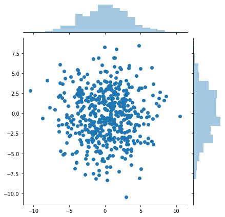
   Figure 1.7 – Joint distribution plot of a multi-dimensional continuous policy

6. Now, we are ready to implement the continuous policy class:

   class ContinuousPolicy(object):
       def __init__(self, action_dim):
           self.action_dim = action_dim
       def sample(self, mu, var):
           self.distribution = \
               tfp.distributions.Normal(loc=mu, scale=sigma)
           return self.distribution.sample(1)
       def get_action(self, mu, var):
           action = self.sample(mu, var)
           return action

7. As a next step, let's implement a multi-dimensional continuous policy class:

   import tensorflow_probability as tfp
   import numpy as np
   class ContinuousMultiDimensionalPolicy(object):
       def __init__(self, num_actions):
           self.action_dim = num_actions
       def sample(self, mu, covariance_diag):
           self.distribution = tfp.distributions.\
                            MultivariateNormalDiag(loc=mu,
                            scale_diag=covariance_diag)
           return self.distribution.sample(1)
       def get_action(self, mu, covariance_diag):
           action = self.sample(mu, covariance_diag)
           return action

8. Let's now implement a function to evaluate an agent in an environment with a continuous action space to assess episodic performance:

   def evaluate(agent, env, render=True):
       obs, episode_reward, done, step_num = env.reset(),
                                             0.0, False, 0
       while not done:
           action = agent.get_action(obs)
           obs, reward, done, info = env.step(action)
           episode_reward += reward
           step_num += 1
           if render:
               env.render()
       return step_num, episode_reward, done, info

9. We are now ready to test the agent in a continuous action environment:

   from neural_agent import Brain
   import gym
   env = gym.make("MountainCarContinuous-v0")Implementing a Neural-network Brain class using TensorFlow 2.x. 
             class Brain(keras.Model):
       def __init__(self, action_dim=5, 
                    input_shape=(1, 8 * 8)):
           """Initialize the Agent's Brain model
           Args:
               action_dim (int): Number of actions
           """
           super(Brain, self).__init__()
           self.dense1 = layers.Dense(32, 
                 input_shape=input_shape, activation="relu")
           self.logits = layers.Dense(action_dim)
       def call(self, inputs):
           x = tf.convert_to_tensor(inputs)
           if len(x.shape) >= 2 and x.shape[0] != 1:
               x = tf.reshape(x, (1, -1))
           return self.logits(self.dense1(x))
       def process(self, observations):
           # Process batch observations using `call(inputs)`
           # behind-the-scenes
           action_logits = \
               self.predict_on_batch(observations)
           return action_logits

10. Let's implement a simple agent class that utilizes the ContinuousPolicy object to act in continuous action space environments:

    class Agent(object):
        def __init__(self, action_dim=5, 
                     input_dim=(1, 8 * 8)):
            self.brain = Brain(action_dim, input_dim)
            self.policy = ContinuousPolicy(action_dim)
        def get_action(self, obs):
            action_logits = self.brain.process(obs)
            action = self.policy.get_action(*np.\
                            squeeze(action_logits, 0))
            return action

11. As a final step, we will test the performance of the agent in a continuous action space environment:

    from neural_agent import Brain
    import gym
    env = gym.make("MountainCarContinuous-v0") 
    action_dim = 2 * env.action_space.shape[0]  
        # 2 values (mu & sigma) for one action dim
    agent = Agent(action_dim, env.observation_space.shape)
    steps, reward, done, info = evaluate(agent, env)
    print(f"steps:{steps} reward:{reward} done:{done} info:{info}")
    env.close()

    The preceding script will call the MountainCarContinuous environment, render it to the screen, and show how the agent is performing in this continuous action space environment:

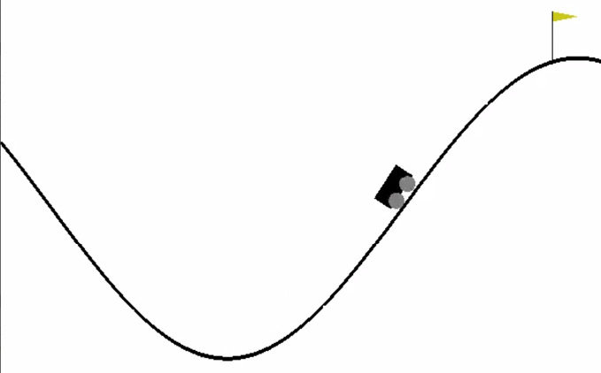
Figure 1.8 – A screenshot of the agent in the MountainCarContinuous-v0 environment

Next, let's explore how it works.

How it works…

We implemented a continuous-valued policy for RL agents using a Gaussian distribution. Gaussian distribution, which is also known as normal distribution, is the most widely used distribution for real numbers. It is represented using two parameters, µ and σ. We generated continuous-valued actions from such a policy by sampling from the distribution, based on the probability density that is given by the following equation:

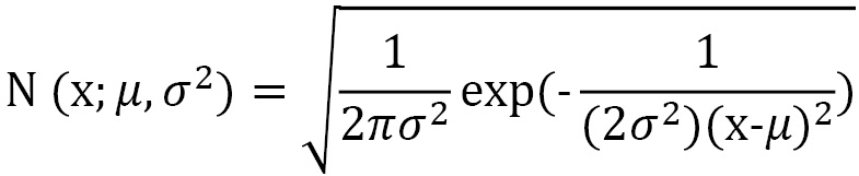
The multivariate normal distribution extends the normal distribution to multiple variables. We used this distribution to generate multi-dimensional continuous policies.