


Training a neural network using PyTorch
For this exercise, we will be using the famous MNIST dataset (available at http://yann.lecun.com/exdb/mnist/), which is a sequence of images of handwritten postcode digits, zero through nine, with corresponding labels. The MNIST dataset consists of 60,000 training samples and 10,000 test samples, where each sample is a grayscale image with 28 x 28 pixels. PyTorch also provides the MNIST dataset under its Dataset module.
In this exercise, we will use PyTorch to train a deep learning multi-class classifier on this dataset and test how the trained model performs on the test samples:
- For this exercise, we will need to import a few dependencies. Execute the following
importstatements:import torch import torch.nn as nn import torch.nn.functional as F import torch.optim as optim from torch.utils.data import DataLoader from torchvision import datasets, transforms import matplotlib.pyplot as plt
- Next, we define the model architecture as shown in the following diagram:
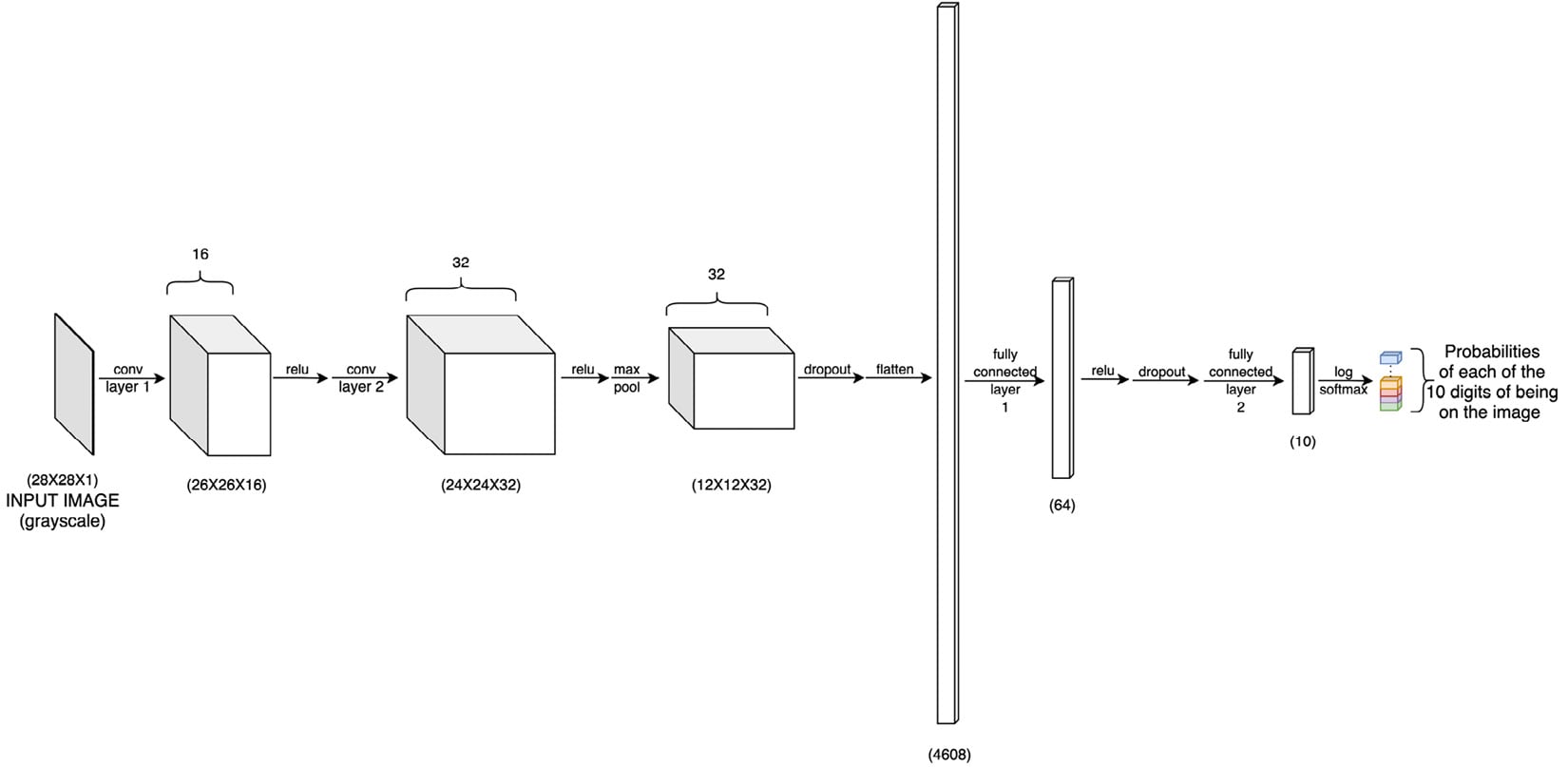
Figure 1.19 – Neural network architecture
The model consists of convolutional layers, dropout layers, as well as linear/fully connected layers, all available through the
torch.nnmodule:class ConvNet(nn.Module): def __init__(self): super(ConvNet, self).__init__() self.cn1 = nn.Conv2d(1, 16, 3, 1) self.cn2 = nn.Conv2d(16, 32, 3, 1) self.dp1 = nn.Dropout2d(0.10) self.dp2 = nn.Dropout2d(0.25) self.fc1 = nn.Linear(4608, 64) # 4608 is basically 12 X 12 X 32 self.fc2 = nn.Linear(64, 10) def forward(self, x): x = self.cn1(x) x = F.relu(x) x = self.cn2(x) x = F.relu(x) x = F.max_pool2d(x, 2) x = self.dp1(x) x = torch.flatten(x, 1) x = self.fc1(x) x = F.relu(x) x = self.dp2(x) x = self.fc2(x) op = F.log_softmax(x, dim=1) return op
The
__init__function defines the core architecture of the model, that is, all the layers with the number of neurons at each layer. And theforwardfunction, as the name suggests, does a forward pass in the network. Hence it includes all the activation functions at each layer as well as any pooling or dropout used after any layer. This function shall return the final layer output, which we call the prediction of the model, which has the same dimensions as the target output (the ground truth).Notice that the first convolutional layer has a 1-channel input, a 16-channel output, a kernel size of 3, and a stride of 1. The 1-channel input is essentially for the grayscale images that will be fed to the model. We decided on a kernel size of 3x3 for various reasons. Firstly, kernel sizes are usually odd numbers so that the input image pixels are symmetrically distributed around a central pixel. 1x1 would be too small because then the kernel operating on a given pixel would not have any information about the neighboring pixels. 3 comes next, but why not go further to 5, 7, or, say, even 27?
Well, at the extreme high end, a 27x27 kernel convolving over a 28x28 image would give us very coarse-grained features. However, the most important visual features in the image are fairly local and hence it makes sense to use a small kernel that looks at a few neighboring pixels at a time, for visual patterns. 3x3 is one of the most common kernel sizes used in CNNs for solving computer vision problems.
Note that we have two consecutive convolutional layers, both with 3x3 kernels. This, in terms of spatial coverage, is equivalent to using one convolutional layer with a 5x5 kernel. However, using multiple layers with a smaller kernel size is almost always preferred because it results in deeper networks, hence more complex learned features as well as fewer parameters due to smaller kernels.
The number of channels in the output of a convolutional layer is usually higher than or equal to the input number of channels. Our first convolutional layer takes in one channel data and outputs 16 channels. This basically means that the layer is trying to detect 16 different kinds of information from the input image. Each of these channels is called a feature map and each of them has a dedicated kernel extracting features for them.
We escalate the number of channels from 16 to 32 in the second convolutional layer, in an attempt to extract more kinds of features from the image. This increment in the number of channels (or image depth) is common practice in CNNs. We will read more on this under width-based CNNs in Chapter 3, Deep CNN Architectures.
Finally, the stride of
1makes sense, as our kernel size is just3. Keeping a larger stride value – say, 10 – would result in the kernel skipping many pixels in the image and we don't want to do that. If, however, our kernel size was 100, we might have considered 10 as a reasonable stride value. The larger the stride, the lower the number of convolution operations but the smaller the overall field of view for the kernel. - We then define the training routine, that is, the actual backpropagation step. As can be seen, the
torch.optimmodule greatly helps in keeping this code succinct:def train(model, device, train_dataloader, optim, epoch): model.train() for b_i, (X, y) in enumerate(train_dataloader): X, y = X.to(device), y.to(device) optim.zero_grad() pred_prob = model(X) loss = F.nll_loss(pred_prob, y) # nll is the negative likelihood loss loss.backward() optim.step() if b_i % 10 == 0: print('epoch: {} [{}/{} ({:.0f}%)]\t training loss: {:.6f}'.format( epoch, b_i * len(X), len(train_ dataloader.dataset), 100. * b_i / len(train_dataloader), loss. item()))This iterates through the dataset in batches, makes a copy of the dataset on the given device, makes a forward pass with the retrieved data on the neural network model, computes the loss between the model prediction and the ground truth, uses the given optimizer to tune model weights, and prints training logs every 10 batches. The entire procedure done once qualifies as
1epoch, that is, when the entire dataset has been read once. - Similar to the preceding training routine, we write a test routine that can be used to evaluate the model performance on the test set:
def test(model, device, test_dataloader):
    model.eval()
    loss = 0
    success = 0
    with torch.no_grad():
        for X, y in test_dataloader:
            X, y = X.to(device), y.to(device)
            pred_prob = model(X)
            loss += F.nll_loss(pred_prob, y, reduction='sum').item()  # loss summed across the batch
            pred = pred_prob.argmax(dim=1, 		 keepdim=True)  # us argmax to get the most 		 likely prediction
            success += pred.eq(y.view_as(pred)).sum().item()
    loss /= len(test_dataloader.dataset)
    print('\nTest dataset: Overall Loss: {:.4f}, Overall Accuracy: {}/{} ({:.0f}%)\n'.format(
        loss, success, len(test_dataloader.dataset),
        100. * success / len(test_dataloader.dataset)))
Most of this function is similar to the preceding
trainfunction. The only difference is that the loss computed from the model predictions and the ground truth is not used to tune the model weights using an optimizer. Instead, the loss is used to compute the overall test error across the entire test batch. - Next, we come to another critical component of this exercise, which is loading the dataset. Thanks to PyTorch's
DataLoadermodule, we can set up the dataset loading mechanism in a few lines of code:# The mean and standard deviation values are calculated as the mean of all pixel values of all images in the training dataset train_dataloader = torch.utils.data.DataLoader( datasets.MNIST('../data', train=True, download=True, transform=transforms.Compose([ transforms.ToTensor(), transforms.Normalize((0.1302,), (0.3069,))])), # train_X.mean()/256. and train_X.std()/256. batch_size=32, shuffle=True) test_dataloader = torch.utils.data.DataLoader( datasets.MNIST('../data', train=False, transform=transforms.Compose([ transforms.ToTensor(), transforms.Normalize((0.1302,), (0.3069,)) ])), batch_size=500, shuffle=False)As you can see, we set
batch_sizeto32, which is a fairly common choice. Usually, there is a trade-off in deciding the batch size. A very small batch size can lead to slow training due to frequent gradient calculations and can lead to extremely noisy gradients. Very large batch sizes can, on the other hand, also slow down training due to a long waiting time to calculate gradients. It is mostly not worth waiting long before a single gradient update. It is rather advisable to make frequent, less precise gradients as it will eventually lead the model to a better set of learned parameters.For both the training and test dataset, we specify the local storage location we want to save the dataset to, and the batch size, which determines the number of data instances that constitute one pass of a training and test run. We also specify that we want to randomly shuffle training data instances to ensure a uniform distribution of data samples across batches. Finally, we also normalize the dataset to a normal distribution with a specified mean and standard deviation.
- We defined the training routine earlier. Now is the time to actually define which optimizer and device we will use to run the model training. And we will finally get the following:
torch.manual_seed(0)
device = torch.device("cpu")
model = ConvNet()
optimizer = optim.Adadelta(model.parameters(), lr=0.5)
We define the device for this exercise as
cpu. We also set a seed to avoid unknown randomness and ensure repeatability. We will use AdaDelta as the optimizer for this exercise with a learning rate of0.5. While discussing optimization schedules earlier in the chapter, we mentioned that Adadelta could be a good choice if we are dealing with sparse data. And this is a case of sparse data, because not all pixels in the image are informative. Having said that, I encourage you to try out other optimizers such as Adam on this same problem to see how it affects the training process and model performance. - And then we start the actual process of training the model for k number of epochs, and we also keep testing the model at the end of each training epoch:
for epoch in range(1, 3):
    train(model, device, train_dataloader, optimizer, epoch)
    test(model, device, test_dataloader)
For demonstration purposes, we will run the training for only two epochs. The output will be as follows:
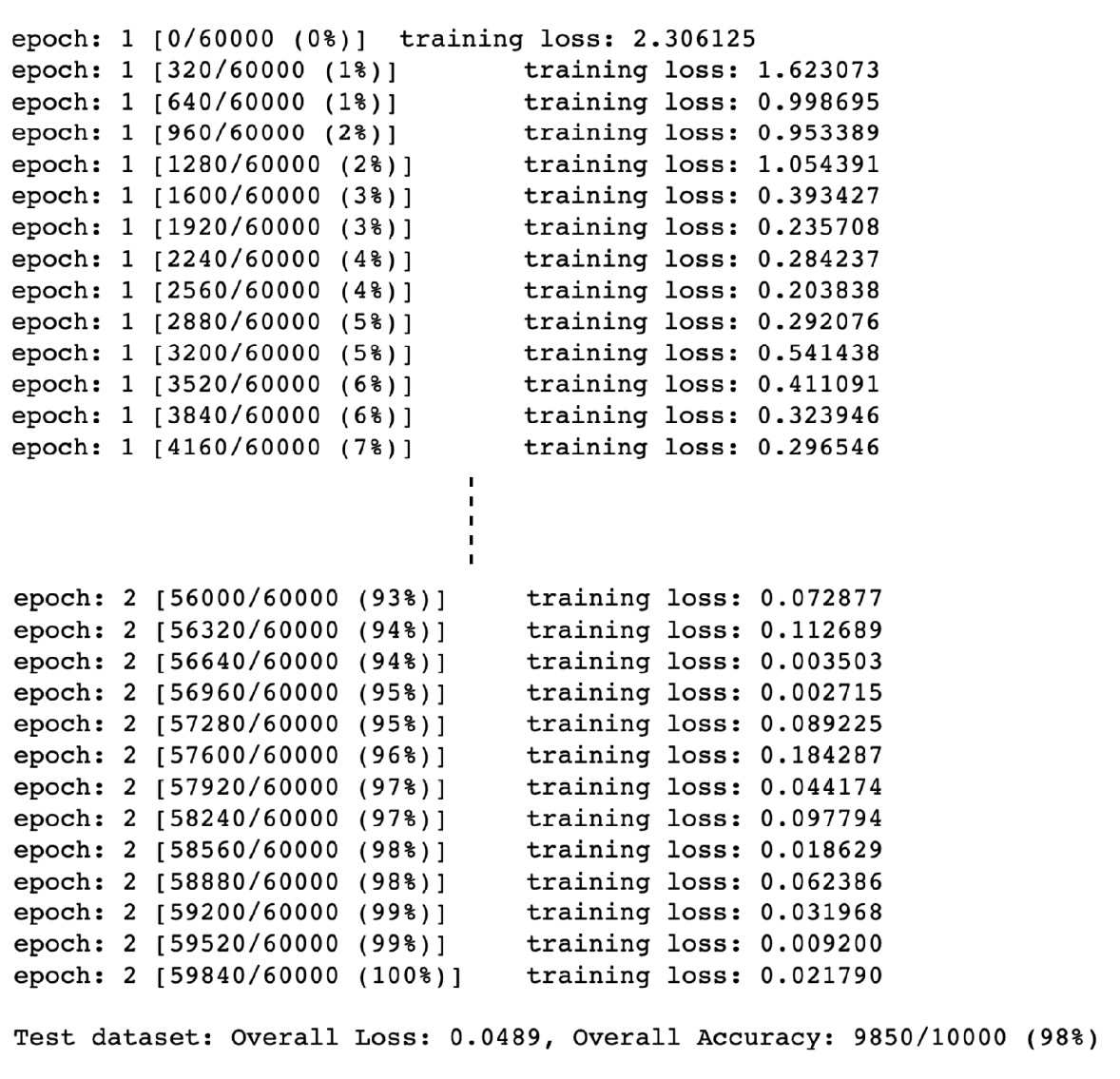
Figure 1.20 – Training logs
- Now that we have trained a model, with a reasonable test set performance, we can also manually check whether the model inference on a sample image is correct:
test_samples = enumerate(test_dataloader)
b_i, (sample_data, sample_targets) = next(test_samples)
plt.imshow(sample_data[0][0], cmap='gray', interpolation='none')
The output will be as follows:
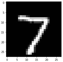
Figure 1.21 – Sample handwritten image
And now we run the model inference for this image and compare it with the ground truth:
     print(f"Model prediction is : {model(sample_data).data.max(1)[1][0]}")
print(f"Ground truth is : {sample_targets[0]}")
Note that, for predictions, we first calculate the class with maximum probability using the max function on axis=1. The max function outputs two lists – a list of probabilities of classes for every sample in sample_data and a list of class labels for each sample. Hence, we choose the second list using index [1]. We further select the first class label by using index [0] to look at only the first sample under sample_data. The output will be as follows:

Figure 1.22 – PyTorch model prediction
This appears to be the correct prediction. The forward pass of the neural network done using model() produces probabilities. Hence, we use the max function to output the class with the maximum probability.
Note
The code pattern for this exercise is derived from the official PyTorch examples repository, which can be found here: https://github.com/pytorch/examples/tree/master/mnist.