Chapter 3. Graphics with matplotlib

This chapter explores matplotlib, an IPython library for production of publication-quality graphs. In this chapter, the following topics will be discussed:

• Two-dimensional plots using the plot function and setting up line widths, colors, and styles

• Plot configuration and annotation

• Three-dimensional plots

• Animations

Being an IPython library, matplotlib consists of a hierarchy of classes, and it is possible to code using it in the usual object-oriented style. However, matplotlib also supports an interactive mode. In this mode, the graphs are constructed step-by-step, thus adding and configuring each component at a time. We lay emphasis on the second approach since it is designed for the rapid production of graphs. The object-oriented style will be explained whenever it is needed or leads to better results.

Note

The sense in which the word interactive is used in this context is somewhat different from what is understood today. Graphs produced by matplotlib are...

The plot function

The plot() function is the workhorse of the matplotlib library. In this section, we will explore the line-plotting and formatting capabilities included in this function.

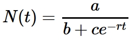
To make things a bit more concrete, let's consider the formula for logistic growth, as follows:

This model is frequently used to represent growth that shows an initial exponential phase, and then is eventually limited by some factor. The examples are the population in an environment with limited resources and new products and/or technological innovations, which initially attract a small and quickly growing market but eventually reach a saturation point.

A common strategy to understand a mathematical model is to investigate how it changes as the parameters defining it are modified. Let's say, we want to see what happens to the shape of the curve when the parameter b changes.

To be able to do what we want more efficiently, we are going to use a function factory. This way, we can quickly create logistic models...

Three-dimensional plots

In this section, we present methods to display three-dimensional plots, that is, plots of mathematical objects in space. Examples include surfaces and lines that are not confined to a plate.

matplotlib has excellent support for three-dimensional plots. In this section, we will present an example of a surface plot and corresponding contour plot. The types of plot available in the three-dimensional library include wireframe plots, line plots, scatterplots, triangulated surface plots, polygon plots, and several others. The following link will help you to understand the types of plots that are not treated here: http://matplotlib.org/1.3.1/mpl_toolkits/mplot3d/tutorial.html#mplot3d-tutorial

Before we start, we need to import the three-dimensional library objects we need using the following command line:

from mpl_toolkits.mplot3d import axes3d

Now, let's draw our surface plot by running the following code in a cell:

def dist(x, y):
    return sqrt(x**2 + y**2) 
def fsurface...

Animations

We will finish the chapter with a more complex example that illustrates the power that matplotlib gives us. We will create an animation of a forced pendulum, a well-known and much studied example of a dynamic system exhibiting deterministic chaos.

Since this section involves more sophisticated code, we will refrain from using pylab and adopt the generally recommended way of importing modules. This makes the code easier to export to a script if we so wish. We also give samples of some of the object-oriented features of matplotlib.

The process of animating a pendulum (or any physical process) is actually very simple: we compute the position of the pendulum at a finite number of times and display the corresponding images in quick succession. So, the code will naturally break down into the following three pieces:

• A function that displays a pendulum in an arbitrary position

• Setting up the computation of the position of the pendulum at an arbitrary time

• The code that actually computes the...

Summary

In this chapter, we learned how to use matplotlib to produce presentation-quality plots. We covered two-dimensional plots and how to set plot options, and annotate and configure plots. You also learned how to add labels, titles, and legends. We also learned how to draw three-dimensional surface plots and how to create simple animations.

In the next chapter, we will explore how to work with data in the notebook using the pandas library.