Convolutional Neural Networks

In the last chapter, we saw how to perform several signal-processing tasks while leveraging the predictive power of feedforward neural networks. This foundational architecture allowed us to introduce many of the basic features that comprise the learning mechanisms of Artificial Neural Networks (ANNs).

In this chapter, we dive deeper to explore another type of ANN, namely the Convolutional Neural Network (CNN), famous for its adeptness at visual tasks such as image recognition, object detection, and semantic segmentation, to name a few. Indeed, the inspiration for these particular architectures also refers back to our own biology. Soon, we will go over the experiments and discoveries of the human race that led to the inspiration for these complex systems that perform so well. The latest iterations of this idea can be traced back to the ImageNet classification...

Why CNNs?

CNNs are very similar to ordinary neural networks. As we have seen in the previous chapter, neural networks are made up of neurons that have learnable weights and biases. Each neuron still computes the weighted sum of its inputs using dot products, adds a bias term, and passes it through a nonlinear equation. The network will show just one differentiable score function that will be, from raw images at one end to the class scores at other end.

And they will also have a loss function such as the softmax, or SVM on the last layer. Moreover, all the techniques that we learned ti develop neural networks will be applicable.

But then what's different with ConvNets you may ask. So the main point to note is that the ConvNet architecture explicitly assumes that the inputs that are received are all images, this assumption actually helps us to encode other properties of the...

The birth of vision

The following is an epic tale, an epic tale that took place nearly 540 million years ago.

Around this time, on the pale blue cosmic dot that would later become known as Earth, life was quite tranquil and hassle-free. Back then, almost all of our ancestors were water dwellers, who would just float about in the serenity of the oceans, munching on sources of food only if they were to float by them. Yes, this was quite different than the predatory, stressful, and stimulating world of today.

Suddenly, something quite curious occurred. In a comparatively short period of time that followed, there was an explosion in the number and variety of animal species present on our planet. In only a span of about 20 million years that came after, the kind of creatures you could find on our watery earth drastically changed. They changed from the occasional single-celled organisms...

Understanding biological vision

Our next insight into biological visual systems comes from a series of experiments conducted by scientists from Harvard University, back in the late 1950s. Nobel laureates David Hubel and Torstein Wiesel showed the world the inner workings of the mammalian visual cortex, by mapping the action of receptor cells along with the visual pathway of a cat, from the retina to the visual cortex. These scientists used electrophysiology to understand exactly how our sensory organs intake, process, and interpret electromagnetic radiation, to generate the reality we see around us. This allowed them to better appreciate the flow of stimuli and related responses that occur at the level of individual neurons:

The following screenshot describes how cells respond to light:

Thanks to their experiments in the field of neuroscience, we are able to share with you several...

Conceptualizing spatial invariance

The first of these notions comes from the concept of spatial invariance. The researchers noticed that the cat's neural activations to particular patterns would be consistent, regardless of the exact location of the patterns on the screen. Intuitively, the same set of neurons were noted to fire for a given pattern (that is, a line segment), even if the pattern appeared at the top or the bottom of the screen. This showed that the neurons' activations were spatially invariant, meaning that their activations were not dependent on the spatial location of the given patterns.

Defining receptive fields of neurons

Secondly, they also noted that neurons were in charge of responding to specific regions of a given input. They named this property of a neuron as its receptive field. In other words, certain neurons only responded to certain regions of a given input, whereas others responded to different regions of the same input. The receptive field of a neuron simply denotes the span of input to which a neuron is likely to respond.

Implementing a hierarchy of neurons

Finally, the researchers were able to demonstrate that a hierarchy of neurons exists in the visual cortex. They showed that lower-level cells are tasked to detect simple visual patterns, such as line segments. The output from these neurons is used in subsequent layers of neurons to construct more and more complex patterns, forming the objects and people we see and interact with. Indeed, modern neuroscience confirms that the structure of the visual cortex is hierarchically organized to perform increasingly complex inferences using the output of previous layers, as illustrated:

The preceding diagram means that recognizing a friend involves detecting the line segments making up their face (V1), using those segments to build shapes and edges (V2), using those shapes and edges to form complex shapes such as eyes and noses (V3), and then leveraging...

The birth of the modern CNN

It wasn't until the 1980s that Heubel and Wiesel's findings were repurposed in the field of computer science. The Neurocognitron (Fukushima, 1980: https://www.rctn.org/bruno/public/papers/Fukushima1980.pdf) leveraged the concept of simple and complex cells by sandwiching layers of one after the other. This ancestor of the modern neural network used the aforementioned alternating layers to sequentially include modifiable parameters (or simple cells), while using pooling layers (or complex cells) to make the network invariant to minor altercations from the simple cells. While intuitive, this architecture was still not powerful enough to capture the intricate complexities present in visual signals.

One of the major breakthroughs followed in 1998, when famed AI researchers, Yan Lecun and Yoshua Bengio, were able to train a CNN, leveraging gradient...

Designing a CNN

Now, armed with the intuition of biological vision, we understand how neurons must be organized hierarchically, to detect simple patterns and use these to progressively build more complex patterns corresponding to real-world objects. We also know that we must implement a mechanism for spatial invariance to allow neurons to deal with similar inputs occurring at different spatial locations of a given image. Finally, we are aware that implementing a receptive field for each neuron is useful to achieve a topographical mapping of neurons to spatial locations in the real world, so that nearby neurons may represent nearby regions in the field of vision.

Dense versus convolutional layer

You will recall from the previous...

The convolution operation

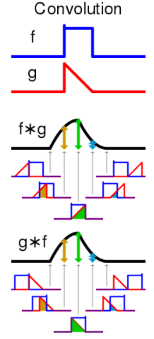
The word convolvere comes from Latin and translates to convolve or roll together. From a mathematical perspective, you may define a convolution as the calculus-based integral denoting the amount by which two given functions overlap, as one of the two is slid across the other. In other words, performing the convolution operation on two functions (f and g) will produce a third function that expresses how the shape of one is modified by the other. The term convolution refers to both the result function and the computation process, with roots in the mathematical subfield of signal processing, as we can here in this diagram:

So, how can we leverage this operation to our advantage?

Preserving the spatial structure of an image

...

Visualizing feature extraction with filters

Let's consider another example, to solidify our understanding of how filters detect patterns. Consider this depiction of the number 7, taken from the MNIST dataset. We use this 28 x 28 pixelated image to show how filters actually pick up on different patterns:

Intuitively, we notice that this 7 is composed of two horizontal lines, as well as a slanted vertical line. We essentially need to initialize our filters with values that can pick up on these separate patterns. Next, we observe some 3 x 3 filter matrices that a ConvNet would typically learn for the task at hand:

While not very intuitive to visualize, these filters are actually sophisticated edge detectors. To see how they work, let's picture each 0 in our filter weights as the color grey, whereas each value of 1 takes the color white, leaving -1 with the color black...

Looking at complex filters

The following image shows the top nine activation maps per grid, associated with specific inputs, for the second layer of a ConvNet. On the left, you can think of the mini-grids as activations of individual neurons, for given inputs. The corresponding colored grids on the right relate to the inputs these neurons were shown. What we are visualizing here is the kind of input that maximizes the activation of these neurons. We notice that already some pretty-clear circle detector neurons are visible (grid 2, 2), being activated for inputs such as the top of lamp shades and animal eyes:

Similarly, we notice some square-like pattern detectors (grid 4, 4) that seem to activate for images containing door and window frames. As we progressively visualize activation maps for deeper layers in CNNs, we observe even more complex geometric patterns being picked up...

Summarizing the convolution operation

All that we are doing here is applying a set of weights (that is, a filter) to local input spaces for feature extraction. We do this iteratively, moving our filter across the input space in fixed steps, known as a stride. Moreover, the use of different filters allows us to capture different patterns from a given input. Finally, since the filters convolve over the entire image, we are able to spatially share parameters for a given filter. This allows us to use the same filter to detect similar patterns in different locations of the image, relating to the concept of spatial invariance discussed earlier. However, these activation maps that a convolutional layer outputs are essentially abstract high-dimensional representations. We need to implement a mechanism to reduce these representations into more manageable dimensions, before we go ahead...

Understanding pooling layers

A final consideration when using convolutional layers is to do with the idea of stacking simple cells to detect local patterns and complex cells to downsample representations, as we saw earlier with the cat-brain experiments, and the neocognitron. The convolutional filters we saw behave like simple cells by focusing on specific locations on the input and training neurons to fire, given some stimuli from the local regions of our input image. Complex cells, on the other hand, are required to be less specific to the location of the stimuli. This is where the pooling layer comes in. This technique of pooling intends to reduce the output of CNN layers to more manageable representations. Pooling layers are periodically added between convolutional layers to spatially downsample the outputs of our convolutional layer. All this does is progressively reduce...

Implementing CNNs in Keras

Having achieved a high-level understanding of the key components of a CNN, we may now proceed with actually implementing one ourselves. This will allow us to become familiar with the key architectural considerations when building convolutional networks and get an overview of the implementational details that make these networks perform so well. Soon, we will implement the convolutional layer in Keras, and explore downsampling techniques such as pooling layers to see how we can leverage a combination of convolutional, pooling, and densely connected layers for various image classification tasks.

For this example, we will adopt a simple use case. Let's say we wanted our CNN to detect human emotion, in the form of a smile or a frown. This is a simple binary classification task. How do we proceed? Well, firstly, we will need a labeled dataset of humans...

Convolutional layer

Two main architectural considerations are associated with the convolutional layer in Keras. The first is to do with the number of filters to employ in the given layer, whereas the second denotes the size of the filters themselves. So, let's see how this is implemented by initializing a blank sequential model and adding our first convolutional layer to it:

model=sequential()
#First Convolutional layer 
model.add(Conv2D(16,(5,5), padding = 'same', activation = 'relu', input_shape = (64,64,3)))
model.add(BatchNormalization())

Defining the number and size of the filters

As we saw previously, we define the layer by embodying it with 16 filters, each with a height and width of 5 x 5. In...

Leveraging a fully connected layer for classification

Then, we simply add a few more layers of convolution, batch normalization, and dropouts, progressively building our network until we reach the final layers. Just like in the MNIST example, we will leverage densely connected layers to implement the classification mechanism in our network. Before we can do this, we must flatten our input from the previous layer (16 x 16 x 32) to a 1D vector of dimension (8,192). We do this because dense layer-based classifiers prefer to receive 1D vectors, unlike the output from our previous layer. We proceed by adding two densely connected layers, the first one with 128 neurons (an arbitrary choice) and the second one with just one neuron, since we are dealing with a binary classification problem. If everything goes according to plan, this one neuron will be supported by its cabinet of neurons...

Summarizing our model

Let's visualize our model to better understand what we just built. You will notice that the number of activation maps (denoted by the depth of subsequent layer outputs) progressively increases throughout the network. On the other hand, the length and width of the activation maps tend to decrease, from (64 x 64) to (16 x 16), by the time the dropout layer is reached. These two patterns are conventional in most, if not all, modern iterations of CNNs.

The reason behind the variance in input and output dimensions between layers can depend on how you have chosen to address the border effects we discussed earlier, or what stride you have implemented for the filters in your convolutional layer. Smaller strides will lead to higher dimensions, whereas larger strides will lead to lower dimensions. This is simply to do with the number of locations you are computing...

Checking model accuracy

As we saw previously, we achieved a test accuracy of 88% at the last epoch of our training session. Let's have a look at what this really means, by interpreting the precision and recall scores of our classifier:

As we noticed previously, the ratio of correctly predicted positive observations to the total number of positive observations in our test set (otherwise known as the precision score) is pretty high at 0.98. The recall score is a bit lower and denotes the number of correctly predicted results divided by the number of results that should have been returned. Finally, the F-measure simply combines both the precision and recall scores as a harmonic mean.

To supplement our understanding, we plot out a confusion matrix of our classifier on the test set, as shown as follows. This is essentially an error matrix that lets us visualize how our model...

The problem with detecting smiles

We must note at this point, that the problem of external validity (that is, the generalizability of our model) persists with a dataset like the smile detector. Given the restricted manner in which data has been collected, it would be unreasonable to expect our CNN to generalize well on other data. Firstly, the network is trained with low resolution input images. Moreover, it has only seen images of one smiling or frowning person in the same location each time. Feeding this network an image of, say, the managerial board of FIFA will not cause it to detect smiles however large and present they may be. We would need to readapt our approach. One way can be through applying the same transformations to the input image as done for the training data, by segmenting and resizing the input image per face. A better approach would be to gather more varied...

Introducing Keras's functional API

How exactly will we do this? Well we start by importing the Model class from the functional API. This lets us define a new model. The key difference in our new model is that this one is capable of giving us back multiple outputs, pertaining to the outputs of intermediate layers. This is achieved by using the layer outputs from a trained CNN (such as our smile detector) and feed it into this new multi-output model. Essentially, our multi-output model will take an input image and return filter-wise activations for each of the eight layers in our smile detector model that we previously trained.

You can also limit the number of layers to visualize through the list slicing notation used on model.layers, shown as follows:

The last line of the preceding code defines the activations variable, by making our multi-output model perform inference on...

Verifying the number of channels per layer

We saw that each layer has a depth that denoted the number of activation maps. These are also referred to as channels, where each channel contains an activation map, with a height and width of (n x n). Our first layer, for example, has 16 different maps of size 64 x 64. Similarly, the fourth layer has 16 activation maps of size 32 x 32. The eighth layer has 32 activation maps, each of size 16 x 16. Each of these activation maps was generated by a specific filter from its respective layer, and are passed forward to subsequent layers to encode higher-level features. This will concur with our smile detector model's architectural build, which we can always verify, as shown here:

Visualizing activation maps

...

Understanding saliency

We saw earlier that the intermediate layers of our ConvNet seemed to encode some pretty clear detectors of face edges. It is harder to distinguish, however, whether our network understands what a smile actually is. You will notice in our smiling faces dataset that all pictures have been taken on the same background at the same approximate angle from the camera. Moreover, you will notice that the individuals in our dataset tend to smile as they lift their head up high and clear, yet mostly tilt their head downward while frowning. That's a lot of opportunity for our network to overfit on some irrelevant pattern. Hence, how do we actually know that our network understands that a smile has more to do with the movement of a person’s lips than it has to do with the angle at which someone’s face is tilted? As we saw in our neural network fails...

Visualizing saliency maps with ResNet50

To keep things interesting, we will conclude our smile detector experiments and actually use a pre-trained, very deep CNN to demonstrate our leopard example. We also use the Keras vis, which is a great higher-level toolkit to visualize and debug CNNs built on Keras. You can install this package using the pip package manager:

Here, we import the ResNet50 CNN architecture with pretrained weights for the ImageNet dataset. We encourage you to explore other models stored in Keras as well, accessible through keras.applications. We also switch out the Softmax activation for the linear activation function in the last layer of this network using utils.apply_modifications, which rebuilds the network graph to help us visualize the saliency of maps better.

ResNet50 was first introduced as the ILSVRC competition and won first place in 2015. It does...

Loading pictures from a local directory

If you would like to follow along, simply google some nice leopard pictures and store them in a local directory. You can use the image loader from the utils module in Keras vis to resize your images to the target size that the ResNet50 model accepts (that is, images of 224 x 224 pixels):

Since we wish to make the experiment considerably arduous for our network, we purposefully selected pictures of camouflaged leopards to see how well this network does at detecting some of nature's most intricate attempts to hide these predatory creatures from the sight of prey, such as ourselves:

Using Keras's visualization module

Even our biological neural networks implemented throughout our visual cortex seem to have some difficulty finding the leopard in each image, at first glance. Let's see how well its artificial counterpart does at this the task. In the following segment of code, we import the saliency visualizer object from the keras-vis module, as well as a utils tool that lets us search for layers by name. Note that this module does not come with the standard Keras install. However, it can be easily installed using the pip package manager on Python. You can even execute the install through your Jupyter environment:

! pip install keras-vis

Searching through layers

Next, we perform a utility search to define our last densely connected layer in the model. We want this layer as it outputs the class probability scores per output category, which we need to be able to visualize the saliency on the input image. The names of the layer can be found in the summary of the model (model.summary()). We will pass four specific arguments to the visualize_salency() function:

This will return the gradients of our output with respect to our input, which intuitively inform us what pixels have the largest effect on our model's prediction. The gradient variable stores six 224 x 224 images (corresponding to the input size for the ResNet50 architecture), one for each of the six input images of leopards. As we noted, these images are generated by the visualize_salency function, which takes four arguments as input:

• A seed input image...

Exercise

• Probe all the layers in the network. What do you notice?

Gradient weighted class activation mapping

Another nifty gradient-based method is the gradient weighted class activation map (Grad-CAM). This is useful specifically if you have input images with entities belonging to several output classes and you want to visualize which areas in the input picture your network associates most with a specific output class. This technique leverages the class-specific gradient information flowing into the final convolutional layer of a CNN to produce a coarse localization map of the important regions in the image. In other words, we feed our network an input image and take the output activation map of a convolution layer by weighing every channel of the output (that is, the activation maps) by the gradient of the output class with respect to the channel. This allows us to better utilize the spatial information corresponding to what our network pays...

Visualizing class activations with Keras-vis

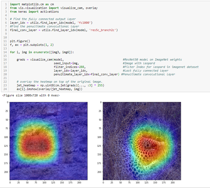
For this purpose, we use the visualize_cam function, which essentially generates a Grad-CAM that maximizes the layer activations for a given input, for a specified output class.

The visualize_cam function takes the same four arguments we saw earlier, plus an additional one. We pass it the arguments corresponding to a Keras model, a seed input image, a filter index corresponding to our output class (ImageNet index for leopard), as well as two model layers. One of these layers remains the fully connected dense output player, whereas the other layer refers to the final convolutional layer in the ResNet50 model. The method essentially leverages these two reference points to generate the gradient weighted class activation maps, as shown:

As we see, the network correctly identifies the leopards in both images. Moreover, we notice that the...

Using the pretrained model for prediction

By the way, you may actually run an inference on a given image using the ResNet50 architecture on pretrained ImageNet weights, as we have initialized here. You can do this by first preprocessing the desired image on which you want to run inference into the appropriate four-dimensional tensor format, as shown here. The same of course applies for any dataset of images you may have, as long as they are resized to the appropriate format:

The preceding code reshapes one of our leopard images into a 4D tensor by expanding its dimension along the 0 axis, then feeds the tensor to our initialized ResNet50 model to get a class probability prediction. We then proceed to decode the prediction class into a human-readable output. For fun, we also defined the labels variable, which includes all the possible labels our network predicted for this image...

Visualizing maximal activations per output class

In the final method, we simply visualize the overall activations associated with a particular output class, without explicitly passing our model an input image. This method can be very intuitive, while being quite aesthetically pleasing. For the purpose of our last experiment, we import yet another pretrained model, the VGG16 network. This network is another deep architecture based on the model that won the ImageNet classification challenge in 2014. Similar to our last example, we switch out the Softmax activation of our last layer with a linear one:

Then, we simply import the activation visualizer object from the visualization module implemented in keras-vis. We plot out the overall activations for the leopard class, by passing the visualize_activation function our model, the output layer, and the index corresponding to our output...

Converging a model

Next, you can make the model converge on this output class to visualize what the model thinks is a leopard (or another output class) after many iterations of convergence. You can define how long you want your model to converge through the max_iter argument, as shown here:

Using multiple filter indices to hallucinate

You can also play around by passing the filter_indices parameter different indices corresponding to different output classes from the ImageNet dataset. You could also pass it a list of two integers, corresponding to two different output classes. This basically lets your neural network imagine visual combinations of two separate output classes by simultaneously visualizing the activations pertaining to both output classes. These can at times turn out to be very interesting, so let both your imaginations run wild! It is noteworthy that Google's DeepDream leverages similar concepts, showing how overexcited activation maps can be superimposed over input images to generate artistic patterns and images. The intricacy of these patterns is at times remarkable and awe-inspiring:

Picture of the author of this book, taken in front of the...

Problems with CNNs

Many may claim that the hierarchically nested pattern recognition technique leveraged by CNNs very much resembles the functioning of our own visual cortex. This may be true at a certain level. However, the visual cortex implements a much more complex architecture and makes it run efficiently on about 10 watts of energy. Our visual cortex also does not easily get fooled by images where face-like features appear, (although this phenomenon occurs often enough to have secured its proper term in modern neuroscience. Pareidolia is a term associated with the human mind interpreting signals in a manner to generate higher-level concepts, where none actually exists. Scientists have shown how this phenomenon is related to the earlier activation of neurons located in the fusiform gyrus area of the visual cortex, responsible for several visual recognition and classification...

Neural network pareidolia

This problem is naturally not unique to our biological brains. In fact, despite the excellent functioning of CNNs for many visual tasks, this problem of neural network pareidolia is one that computer vision researchers are always trying to solve. As we noted, CNNs learn to classify images through learning an assortment of filters that pick up useful features, capable of breaking down the input image in a probabilistic manner. However, the features learned by these filters do not represent all the information present in a given image. The orientation of these features, with respect to one another, matters just as much! The presence of two eyes, lips, and a nose does not inherently constitute the essence of a face. Rather, it's the spatial arrangement of these elements within an image that makes the face in question:

...

Summary

In this chapter, firstly, we used convolutional layers that are capable of decomposing a given visual input space into hierarchically nested probabilistic activations of convolution filters that subsequently connect to dense neurons that perform classification. The filters in these convolutional layers learn weights corresponding to useful representations that may be queried in a probabilistic manner to map the set of input features present in a dataset to the respective output classes. Furthermore, we saw how we can dive deep into our convolution network to understand what it has learned. We saw four specific ways to do this: intermediate activation-based, saliency-based, gradient weighted class activations, and activation maximization visualizations. Each gives a unique intuition into which patterns are picked up by the different layers of our network. We visualized...