Search icon
Arrow left icon
All Products
Best Sellers
New Releases
Books
Videos
Audiobooks
Learning Hub
Newsletters
Free Learning
Arrow right icon
Hands-On GPU Programming with Python and CUDA

Hands-On GPU Programming with Python and CUDA: Explore high-performance parallel computing with CUDA

By Dr. Brian Tuomanen
$48.99
Book Nov 2018 310 pages 1st Edition
eBook
$39.99 $27.98
Print
$48.99
Subscription
$15.99 Monthly
eBook
$39.99 $27.98
Print
$48.99
Subscription
$15.99 Monthly

What do you get with Print?

Product feature icon Instant access to your digital eBook copy whilst your Print order is Shipped
Product feature icon Black & white paperback book shipped to your address
Product feature icon Download this book in EPUB and PDF formats
Product feature icon Access this title in our online reader with advanced features
Product feature icon DRM FREE - Read whenever, wherever and however you want
Buy Now

Product Details


Publication date : Nov 27, 2018
Length 310 pages
Edition : 1st Edition
Language : English
ISBN-13 : 9781788993913
Category :
Table of content icon View table of contents Preview book icon Preview Book

Hands-On GPU Programming with Python and CUDA

Why GPU Programming?

It turns out that besides being able to render graphics for video games, graphics processing units (GPUs) also provide a readily accessible means for the general consumer to do massively parallel computing—an average person can now buy a $2,000 modern GPU card from a local electronics store, plug it into their PC at home, and then use it almost immediately for computational power that would only have been available in the supercomputing labs of top corporations and universities only 5 or 10 years ago. This open accessibility of GPUs has become apparent in many ways in recent years, which can be revealed by a brief observation of the news—cryptocurrency miners use GPUs to generate digital money such as Bitcoins, geneticists and biologists use GPUs for DNA analysis and research, physicists and mathematicians use GPUs for large-scale simulations, AI researchers can now program GPUs to write plays and compose music, while major internet companies, such as Google and Facebook, use farms of servers with GPUs for large-scale machine learning tasks… the list goes on and on.

This book is primarily aimed at bringing you up to speed with GPU programming, so that you too may begin using their power as soon as possible, no matter what your end goal is. We aim to cover the core essentials of how to program a GPU, rather than provide intricate technical details and schematics of how a GPU works. Toward the end of the book, we will provide further resources so that you may specialize further, and apply your new knowledge of GPUs. (Further details as to particular required technical knowledge and hardware follow this section.)

In this book, we will be working with CUDA, a framework for general-purpose GPU (GPGPU) programming from NVIDIA, which was first released back in 2007. While CUDA is proprietary for NVIDIA GPUs, it is a mature and stable platform that is relatively easy to use, provides an unmatched set of first-party accelerated mathematical and AI-related libraries, and comes with the minimal hassle when it comes to installation and integration. Moreover, there are readily available and standardized Python libraries, such as PyCUDA and Scikit-CUDA, which make GPGPU programming all the more readily accessible to aspiring GPU programmers. For these reasons, we are opting to go with CUDA for this book.

CUDA is always pronounced coo-duh, and never as the acronym C-U-D-A! CUDA originally stood for Compute Unified Device Architecture, but Nvidia has dropped the acronym and now uses CUDA as a proper name written in all-caps.

We will now start our journey into GPU programming with an overview of Amdahl's Law. Amdahl's Law is a simple but effective method to estimate potential speed gains we can get by offloading a program or algorithm onto a GPU; this will help us determine whether it's worth our effort to rewrite our code to make use of the GPU. We will then go over a brief review of how to profile our Python code with the cProfile module, to help us find the bottlenecks in our code.

The learning outcomes for this chapter are as follows:

  • Understand Amdahl's Law
  • Apply Amdahl's Law in the context of your code
  • Using the cProfile module for basic profiling of Python code

Technical requirements

Parallelization and Amdahl's Law

Before we can dive in and unlock the potential of GPUs, we first have to realize where their computational power lies in comparison to a modern Intel/AMD central processing unit (CPU)—the power does not lie in the fact that it has a higher clock speed than a CPU, nor in the complexity or particular design of the individual cores. An individual GPU core is actually quite simplistic, and at a disadvantage when compared to a modern individual CPU core, which use many fancy engineering tricks, such as branch prediction to reduce the latency of computations. Latency refers to the beginning-to-end duration of performing a single computation.

The power of the GPU derives from the fact that there are many, many more cores than in a CPU, which means a huge step forward in throughput. Throughput here refers to the number of computations that can be performed simultaneously. Let's use an analogy to get a better understanding of what this means. A GPU is like a very wide city road that is designed to handle many slower-moving cars at once (high throughput, high latency), whereas a CPU is like a narrow highway that can only admit a few cars at once, but can get each individual car to its destination much quicker (low throughput, low latency).

We can get an idea of the increase in throughput by seeing how many cores these new GPUs have. To give you an idea, the average Intel or AMD CPU has only two to eight cores—while an entry-level, consumer-grade NVIDIA GTX 1050 GPU has 640 cores, and a new top-of-the-line NVIDIA RTX 2080 Ti has 4,352 cores! We can exploit this massive throughput, provided we know how properly to parallelize any program or algorithm we wish to speed up. By parallelize, we mean to rewrite a program or algorithm so that we can split up our workload to run in parallel on multiple processors simultaneously. Let's think about an analogy from real-life.

Suppose that you are building a house and that you already have all of the designs and materials in place. You hire a single laborer, and you estimate it will take 100 hours to construct the house. Let's suppose that this particular house can be built in such a way that the work can be perfectly divided between every additional laborer you hire—that is to say, it will take 50 hours for two laborers, 25 hours for four laborers, and 10 hours for ten laborers to construct the house—the number of hours to construct your house will be 100 divided by the number of laborers you hire. This is an example of a parallelizable task.

We notice that this task is twice as fast to complete for two laborers, and ten times as fast for ten laborers to complete together (that is, in parallel) as opposed to one laborer building the house alone (that is, in serial)—that is, if N is the number of laborers, then it will be N times as fast. In this case, N is known as the speedup of parallelizing our task over the serial version of our task.

Before we begin to program a parallel version of a given algorithm, we often start by coming up with an estimate of the potential speedup that parallelization would bring to our task. This can help us determine whether it is worth expending resources and time writing a parallelization of our program or not. Because real life is more complicated than the example we gave here, it's pretty obvious that we won't be able to parallelize every program perfectly, all of the time—most of the time, only a part of our program will be nicely parallelizable, while the rest will have to run in serial.

Using Amdahl's Law

We will now derive Amdahl's Law, which is a simple arithmetic formula that is used to estimate potential speed gain that may arise from parallelizing some portion of code from a serial program onto multiple processors. We will do this by continuing with our prior analogy of building a house.

Last time, we only considered the actual physical construction of the house as the entire time duration, but now, we will also consider the time it takes to design the house into the time duration for building the house. Suppose that only one person in the world has the ability to design your house—you—and it takes you 100 hours to design the plans for your house. There is no possibility that any other person on the planet can compare to your architectural brilliance, so there is no possibility that this part of the task can be split up at all between other architects—that is, so it will take 100 hours to design your house, regardless of what resources you have or how many people you can hire. So, if you have only one laborer to build your house, the entire time it will take to build your home will be 200 hours—100 hours for you to design it, and 100 hours for a single laborer to build it. If we hire two laborers, this will take 150 hours—the time to design the house will remain at 100 hours, while the construction will take 50 hours. It's clear that the total number of hours to construct the house will be 100 + 100 / N, where N is the number of laborers we hire.

Now, let's step back and think about how much time building the house takes if we hire one laborer—we ultimately use this to determine speedup as we hire additional laborers; that is, how many times faster the process becomes. If we hire a single laborer, we see that it takes the same amount of time to both design and construct the house—100 hours. So, we can say that that the portion of time spent on the design is .5 (50%), and the portion of the time it takes to construct the house is .5 (50%)—of course, both of these portions add up to 1, that is 100%. We want to make comparisons to this as we add laborers—if we have two laborers, the portion of time for the construction is halved, so in comparison to the original serial version of our task, this will take .5 + .5/2 = .75 (75%) of the time of the original task, and .75 x 200 hours is 150 hours, so we can see that this works. Moreover, we can see that if we have N laborers, we can calculate the percentage of time our parallelized construction with N laborers will take which the formula .5 + .5 / N.

Now, let's determine the speedup we are gaining by adding additional laborers. Since it takes 75% of the time to build a house if we have two laborers, we can take the reciprocal of .75 to determine the speedup of our parallelization—that is, the speedup will be 1 / .75, which is around 1.33 times faster than if we only have one laborer. In this case, we see that the speedup will be 1 / (.5 + .5 / N) if we have N laborers.

We know that .5 / N will shrink very close to 0 as we add more and more laborers, so we can see there is always an upper bound on the speedup you can get when you parallelize this task—that is, 1 / (.5 + 0) = 2. We can divide the original serial time with the estimated maximum speedup to determine an absolute minimum amount of time this task will take—200 / 2 = 100 hours.

The principle we have just applied to determine speedups in parallel programming is known as Amdahl's Law. It only requires knowledge of the parallelizable proportion of execution time for code in our original serial program, which is referred to as p, and the number of processor cores N that we have available.

The proportion of execution time for code that is not parallelizable in this case is always 1 – p, so we only need to know p.

We can now calculate speedup with Amdahl's Law as follows:

To sum it up, Amdahl's Law is a simple formula that allows us to roughly (very roughly) estimate potential speedup for a program that can be at least partially parallelized. This can provide a general idea as to whether it will be worthwhile to write a parallel version of a particular serial program, provided we know what proportion of the code we can parallelize (p), and how many cores we can run our parallelized code on (N).

The Mandelbrot set

We are now prepared to see a very standard example for parallel computing that we will revisit later in this text—an algorithm to generate an image of the Mandelbrot set. Let's first define exactly what we mean.

For a given complex number, c, we define a recursive sequence for , with and for . If |zn| remains bounded by 2 as n increases to infinity, then we will say that c is a member of the Mandelbrot set.

Recall that we can visualize the complex numbers as residing on a two-dimensional Cartesian plane, with the x-axis representing the real components and the y-axis representing the imaginary components. We can therefore easily visualize the Mandelbrot set with a very appealing (and well-known) graph. Here, we will represent members of the Mandelbrot set with a lighter shade, and nonmembers with a darker shade on the complex Cartesian plane as follows:

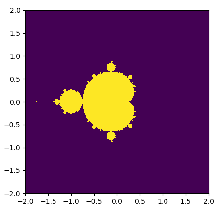
Now, let's think about how we would go about generating this set in Python. We have to consider a few things first—since we obviously can't check whether every single complex number is in the Mandelbrot set, we have to choose a certain range to check over; we have to determine how many points in each range we will consider (width, height); and the maximum value of n that we will check |zn| for (max_iters). We can now prepare to implement a function to generate a graph of the Mandelbrot set—here, we do this by iterating over every single point in the graph in serial.

We will start by importing the NumPy library, which is a numerical library that we will be making ample use of throughout this text. Our implementation here is in the simple_mandelbrot function. We start by using NumPy's linspace function to generate a lattice that will act as a discrete complex plane (the rest of the code that follows should be fairly straightforward):

import numpy as np

def simple_mandelbrot(width, height, real_low, real_high, imag_low, imag_high, max_iters):

real_vals = np.linspace(real_low, real_high, width)
imag_vals = np.linspace(imag_low, imag_high, height)

# we will represent members as 1, non-members as 0.

mandelbrot_graph = np.ones((height,width), dtype=np.float32)

for x in range(width):

for y in range(height):

c = np.complex64( real_vals[x] + imag_vals[y] * 1j )
z = np.complex64(0)

for i in range(max_iters):

z = z**2 + c

if(np.abs(z) > 2):
mandelbrot_graph[y,x] = 0
break

return mandelbrot_graph

Now, we want to add some code to dump the image of the Mandelbrot set to a PNG format file, so let's add the appropriate headers at the beginning:

from time import time
import matplotlib
# the following will prevent the figure from popping up
matplotlib.use('Agg')
from matplotlib import pyplot as plt

Now, let's add some code to generate the Mandelbrot set and dump it to a file, and use the time function to time both operations:

if __name__ == '__main__':

t1 = time()
mandel = simple_mandelbrot(512,512,-2,2,-2,2,256, 2)
t2 = time()
mandel_time = t2 - t1

t1 = time()
fig = plt.figure(1)
plt.imshow(mandel, extent=(-2, 2, -2, 2))
plt.savefig('mandelbrot.png', dpi=fig.dpi)
t2 = time()

dump_time = t2 - t1

print 'It took {} seconds to calculate the Mandelbrot graph.'.format(mandel_time)
print 'It took {} seconds to dump the image.'.format(dump_time)

Now let's run this program (this is also available as the mandelbrot0.py file, in folder 1, within the GitHub repository):

It took about 14.62 seconds to generate the Mandelbrot set, and about 0.11 seconds to dump the image. As we have seen, we generate the Mandelbrot set point by point; there is no interdependence between the values of different points, and it is, therefore, an intrinsically parallelizable function. In contrast, the code to dump the image cannot be parallelized.

Now, let's analyze this in terms of Amdahl's Law. What sort of speedups can we get if we parallelize our code here? In total, both pieces of the program took about 14.73 seconds to run; since we can parallelize the Mandelbrot set generation, we can say that the portion of execution time for parallelizable code is p = 14.62 / 14.73 = .99. This program is 99% parallelizable!

What sort of speedup can we potentially get? Well, I'm currently working on a laptop with an entry-level GTX 1050 GPU with 640 cores; our N will thus be 640 when we use the formula. We calculate the speedup as follows:

That is definitely very good and would indicate to us that it is worth our effort to program our algorithm to use the GPU. Keep in mind that Amdahl's Law only gives a very rough estimate! There will be additional considerations that will come into play when we offload computations onto the GPU, such as the additional time it takes for the CPU to send and receive data to and from the GPU; or the fact that algorithms that are offloaded to the GPU are only partially parallelizable.

Profiling your code

We saw in the previous example that we can individually time different functions and components with the standard time function in Python. While this approach works fine for our small example program, this won't always be feasible for larger programs that call on many different functions, some of which may or may not be worth our effort to parallelize, or even optimize on the CPU. Our goal here is to find the bottlenecks and hotspots of a programeven if we were feeling energetic and used time around every function call we make, we might miss something, or there might be some system or library calls that we don't even consider that happen to be slowing things down. We should find candidate portions of the code to offload onto the GPU before we even think about rewriting the code to run on the GPU; we must always follow the wise words of the famous American computer scientist Donald Knuth: Premature optimization is the root of all evil.

We use what is known as a profiler to find these hot spots and bottlenecks in our code. A profiler will conveniently allow us to see where our program is taking the most time, and allow us to optimize accordingly.

Using the cProfile module

We will primarily be using the cProfile module to check our code. This module is a standard library function that is contained in every modern Python installation. We can run the profiler from the command line with -m cProfile, and specify that we want to organize the results by the cumulative time spent on each function with -s cumtime, and then redirect the output into a text file with the > operator.

This will work on both the Linux Bash or Windows PowerShell command line.

Let's try this now:

We can now look at the contents of the text file with our favorite text editor. Let's keep in mind that the output of the program will be included at the beginning of the file:

Now, since we didn't remove the references to time in the original example, we see their output in the first two lines at the beginning. We can then see the total number of function calls made in this program, and the cumulative amount of time to run it.

Subsequently, we have a list of functions that are called in the program, ordered from the cumulatively most time-consuming functions to the least; the first line is the program itself, while the second line is, as expected, the simple_mandelbrot function from our program. (Notice that the time here aligns with what we measured with the time command). After this, we can see many libraries and system calls that relate to dumping the Mandelbrot graph to a file, all of which take comparatively less time. We use such output from cProfile to infer where our bottlenecks are within a given program.

Summary

The main advantage of using a GPU over a CPU is its increased throughput, which means that we can execute more parallel code simultaneously on GPU than on a CPU; a GPU cannot make recursive algorithms or nonparallelizable algorithms somewhat faster. We see that some tasks, such as the example of building a house, are only partially parallelizable—in this example, we couldn't speed up the process of designing the house (which is intrinsically serial in this case), but we could speed up the process of the construction, by hiring more laborers (which is parallelizable in this case).

We used this analogy to derive Amdahl's Law, which is a formula that can give us a rough estimate of potential speedup for a program if we know the percentage of execution time for code that is parallelizable, and how many processors we will have to run this code. We then applied Amdahl's Law to analyze a small program that generates the Mandelbrot set and dumps it to an image file, and we determined that this would be a good candidate for parallelization onto a GPU. Finally, we ended with a brief overview of profiling code with the cPython module; this allows us to see where the bottlenecks in a program are, without explicitly timing function calls.

Now that we have a few of the fundamental concepts in place, and have a motivator to learn GPU programming, we will spend the next chapter setting up a Linux- or Windows 10-based GPU programming environment. We will then immediately dive into the world of GPU programming in the following chapter, where we will actually write a GPU-based version of the Mandelbrot program that we saw in this chapter.

Questions

  1. There are three for statements in this chapter's Mandelbrot example; however, we can only parallelize over the first two. Why can't we parallelize over all of the for loops here?
  2. What is something that Amdahl's Law doesn't account for when we apply it to offloading a serial CPU algorithm to a GPU?
  3. Suppose that you gain exclusive access to three new top-secret GPUs that are the same in all respects, except for core counts—the first has 131,072 cores, the second has 262,144 cores, and the third has 524,288 cores. If you parallelize and offload the Mandelbrot example onto these GPUs (which generates a 512 x 512 pixel image), will there be a difference in computation time between the first and second GPU? How about between the second and third GPU?
  4. Can you think of any problems with designating certain algorithms or blocks of code as parallelizable in the context of Amdahl's Law?
  5. Why should we use profilers instead of just using Python's time function?
Left arrow icon Right arrow icon
Download code icon Download Code

Key benefits

  • Expand your background in GPU programming—PyCUDA, scikit-cuda, and Nsight
  • Effectively use CUDA libraries such as cuBLAS, cuFFT, and cuSolver
  • Apply GPU programming to modern data science applications

Description

Hands-On GPU Programming with Python and CUDA hits the ground running: you’ll start by learning how to apply Amdahl’s Law, use a code profiler to identify bottlenecks in your Python code, and set up an appropriate GPU programming environment. You’ll then see how to “query” the GPU’s features and copy arrays of data to and from the GPU’s own memory. As you make your way through the book, you’ll launch code directly onto the GPU and write full blown GPU kernels and device functions in CUDA C. You’ll get to grips with profiling GPU code effectively and fully test and debug your code using Nsight IDE. Next, you’ll explore some of the more well-known NVIDIA libraries, such as cuFFT and cuBLAS. With a solid background in place, you will now apply your new-found knowledge to develop your very own GPU-based deep neural network from scratch. You’ll then explore advanced topics, such as warp shuffling, dynamic parallelism, and PTX assembly. In the final chapter, you’ll see some topics and applications related to GPU programming that you may wish to pursue, including AI, graphics, and blockchain. By the end of this book, you will be able to apply GPU programming to problems related to data science and high-performance computing.

What you will learn

Launch GPU code directly from Python Write effective and efficient GPU kernels and device functions Use libraries such as cuFFT, cuBLAS, and cuSolver Debug and profile your code with Nsight and Visual Profiler Apply GPU programming to datascience problems Build a GPU-based deep neuralnetwork from scratch Explore advanced GPU hardware features, such as warp shuffling

What do you get with Print?

Product feature icon Instant access to your digital eBook copy whilst your Print order is Shipped
Product feature icon Black & white paperback book shipped to your address
Product feature icon Download this book in EPUB and PDF formats
Product feature icon Access this title in our online reader with advanced features
Product feature icon DRM FREE - Read whenever, wherever and however you want
Buy Now

Product Details


Publication date : Nov 27, 2018
Length 310 pages
Edition : 1st Edition
Language : English
ISBN-13 : 9781788993913
Category :

Table of Contents

15 Chapters
Preface Chevron down icon Chevron up icon
Why GPU Programming? Chevron down icon Chevron up icon
Setting Up Your GPU Programming Environment Chevron down icon Chevron up icon
Getting Started with PyCUDA Chevron down icon Chevron up icon
Kernels, Threads, Blocks, and Grids Chevron down icon Chevron up icon
Streams, Events, Contexts, and Concurrency Chevron down icon Chevron up icon
Debugging and Profiling Your CUDA Code Chevron down icon Chevron up icon
Using the CUDA Libraries with Scikit-CUDA Chevron down icon Chevron up icon
The CUDA Device Function Libraries and Thrust Chevron down icon Chevron up icon
Implementation of a Deep Neural Network Chevron down icon Chevron up icon
Working with Compiled GPU Code Chevron down icon Chevron up icon
Performance Optimization in CUDA Chevron down icon Chevron up icon
Where to Go from Here Chevron down icon Chevron up icon
Assessment Chevron down icon Chevron up icon
Other Books You May Enjoy Chevron down icon Chevron up icon

Customer reviews

Filter icon Filter
Top Reviews
Rating distribution
Empty star icon Empty star icon Empty star icon Empty star icon Empty star icon 0
(0 Ratings)
5 star 0%
4 star 0%
3 star 0%
2 star 0%
1 star 0%

Filter reviews by


No reviews found
Get free access to Packt library with over 7500+ books and video courses for 7 days!
Start Free Trial

FAQs

What is the delivery time and cost of print book? Chevron down icon Chevron up icon

Shipping Details

USA:

'

Economy: Delivery to most addresses in the US within 10-15 business days

Premium: Trackable Delivery to most addresses in the US within 3-8 business days

UK:

Economy: Delivery to most addresses in the U.K. within 7-9 business days.
Shipments are not trackable

Premium: Trackable delivery to most addresses in the U.K. within 3-4 business days!
Add one extra business day for deliveries to Northern Ireland and Scottish Highlands and islands

EU:

Premium: Trackable delivery to most EU destinations within 4-9 business days.

Australia:

Economy: Can deliver to P. O. Boxes and private residences.
Trackable service with delivery to addresses in Australia only.
Delivery time ranges from 7-9 business days for VIC and 8-10 business days for Interstate metro
Delivery time is up to 15 business days for remote areas of WA, NT & QLD.

Premium: Delivery to addresses in Australia only
Trackable delivery to most P. O. Boxes and private residences in Australia within 4-5 days based on the distance to a destination following dispatch.

India:

Premium: Delivery to most Indian addresses within 5-6 business days

Rest of the World:

Premium: Countries in the American continent: Trackable delivery to most countries within 4-7 business days

Asia:

Premium: Delivery to most Asian addresses within 5-9 business days

Disclaimer:
All orders received before 5 PM U.K time would start printing from the next business day. So the estimated delivery times start from the next day as well. Orders received after 5 PM U.K time (in our internal systems) on a business day or anytime on the weekend will begin printing the second to next business day. For example, an order placed at 11 AM today will begin printing tomorrow, whereas an order placed at 9 PM tonight will begin printing the day after tomorrow.


Unfortunately, due to several restrictions, we are unable to ship to the following countries:

  1. Afghanistan
  2. American Samoa
  3. Belarus
  4. Brunei Darussalam
  5. Central African Republic
  6. The Democratic Republic of Congo
  7. Eritrea
  8. Guinea-bissau
  9. Iran
  10. Lebanon
  11. Libiya Arab Jamahriya
  12. Somalia
  13. Sudan
  14. Russian Federation
  15. Syrian Arab Republic
  16. Ukraine
  17. Venezuela
What is custom duty/charge? Chevron down icon Chevron up icon

Customs duty are charges levied on goods when they cross international borders. It is a tax that is imposed on imported goods. These duties are charged by special authorities and bodies created by local governments and are meant to protect local industries, economies, and businesses.

Do I have to pay customs charges for the print book order? Chevron down icon Chevron up icon

The orders shipped to the countries that are listed under EU27 will not bear custom charges. They are paid by Packt as part of the order.

List of EU27 countries: www.gov.uk/eu-eea:

A custom duty or localized taxes may be applicable on the shipment and would be charged by the recipient country outside of the EU27 which should be paid by the customer and these duties are not included in the shipping charges been charged on the order.

How do I know my custom duty charges? Chevron down icon Chevron up icon

The amount of duty payable varies greatly depending on the imported goods, the country of origin and several other factors like the total invoice amount or dimensions like weight, and other such criteria applicable in your country.

For example:

  • If you live in Mexico, and the declared value of your ordered items is over $ 50, for you to receive a package, you will have to pay additional import tax of 19% which will be $ 9.50 to the courier service.
  • Whereas if you live in Turkey, and the declared value of your ordered items is over € 22, for you to receive a package, you will have to pay additional import tax of 18% which will be € 3.96 to the courier service.
How can I cancel my order? Chevron down icon Chevron up icon

Cancellation Policy for Published Printed Books:

You can cancel any order within 1 hour of placing the order. Simply contact customercare@packt.com with your order details or payment transaction id. If your order has already started the shipment process, we will do our best to stop it. However, if it is already on the way to you then when you receive it, you can contact us at customercare@packt.com using the returns and refund process.

Please understand that Packt Publishing cannot provide refunds or cancel any order except for the cases described in our Return Policy (i.e. Packt Publishing agrees to replace your printed book because it arrives damaged or material defect in book), Packt Publishing will not accept returns.

What is your returns and refunds policy? Chevron down icon Chevron up icon

Return Policy:

We want you to be happy with your purchase from Packtpub.com. We will not hassle you with returning print books to us. If the print book you receive from us is incorrect, damaged, doesn't work or is unacceptably late, please contact Customer Relations Team on customercare@packt.com with the order number and issue details as explained below:

  1. If you ordered (eBook, Video or Print Book) incorrectly or accidentally, please contact Customer Relations Team on customercare@packt.com within one hour of placing the order and we will replace/refund you the item cost.
  2. Sadly, if your eBook or Video file is faulty or a fault occurs during the eBook or Video being made available to you, i.e. during download then you should contact Customer Relations Team within 14 days of purchase on customercare@packt.com who will be able to resolve this issue for you.
  3. You will have a choice of replacement or refund of the problem items.(damaged, defective or incorrect)
  4. Once Customer Care Team confirms that you will be refunded, you should receive the refund within 10 to 12 working days.
  5. If you are only requesting a refund of one book from a multiple order, then we will refund you the appropriate single item.
  6. Where the items were shipped under a free shipping offer, there will be no shipping costs to refund.

On the off chance your printed book arrives damaged, with book material defect, contact our Customer Relation Team on customercare@packt.com within 14 days of receipt of the book with appropriate evidence of damage and we will work with you to secure a replacement copy, if necessary. Please note that each printed book you order from us is individually made by Packt's professional book-printing partner which is on a print-on-demand basis.

What tax is charged? Chevron down icon Chevron up icon

Currently, no tax is charged on the purchase of any print book (subject to change based on the laws and regulations). A localized VAT fee is charged only to our European and UK customers on eBooks, Video and subscriptions that they buy. GST is charged to Indian customers for eBooks and video purchases.

What payment methods can I use? Chevron down icon Chevron up icon

You can pay with the following card types:

  1. Visa Debit
  2. Visa Credit
  3. MasterCard
  4. PayPal
What is the delivery time and cost of print books? Chevron down icon Chevron up icon

Shipping Details

USA:

'

Economy: Delivery to most addresses in the US within 10-15 business days

Premium: Trackable Delivery to most addresses in the US within 3-8 business days

UK:

Economy: Delivery to most addresses in the U.K. within 7-9 business days.
Shipments are not trackable

Premium: Trackable delivery to most addresses in the U.K. within 3-4 business days!
Add one extra business day for deliveries to Northern Ireland and Scottish Highlands and islands

EU:

Premium: Trackable delivery to most EU destinations within 4-9 business days.

Australia:

Economy: Can deliver to P. O. Boxes and private residences.
Trackable service with delivery to addresses in Australia only.
Delivery time ranges from 7-9 business days for VIC and 8-10 business days for Interstate metro
Delivery time is up to 15 business days for remote areas of WA, NT & QLD.

Premium: Delivery to addresses in Australia only
Trackable delivery to most P. O. Boxes and private residences in Australia within 4-5 days based on the distance to a destination following dispatch.

India:

Premium: Delivery to most Indian addresses within 5-6 business days

Rest of the World:

Premium: Countries in the American continent: Trackable delivery to most countries within 4-7 business days

Asia:

Premium: Delivery to most Asian addresses within 5-9 business days

Disclaimer:
All orders received before 5 PM U.K time would start printing from the next business day. So the estimated delivery times start from the next day as well. Orders received after 5 PM U.K time (in our internal systems) on a business day or anytime on the weekend will begin printing the second to next business day. For example, an order placed at 11 AM today will begin printing tomorrow, whereas an order placed at 9 PM tonight will begin printing the day after tomorrow.


Unfortunately, due to several restrictions, we are unable to ship to the following countries:

  1. Afghanistan
  2. American Samoa
  3. Belarus
  4. Brunei Darussalam
  5. Central African Republic
  6. The Democratic Republic of Congo
  7. Eritrea
  8. Guinea-bissau
  9. Iran
  10. Lebanon
  11. Libiya Arab Jamahriya
  12. Somalia
  13. Sudan
  14. Russian Federation
  15. Syrian Arab Republic
  16. Ukraine
  17. Venezuela