Reader small image

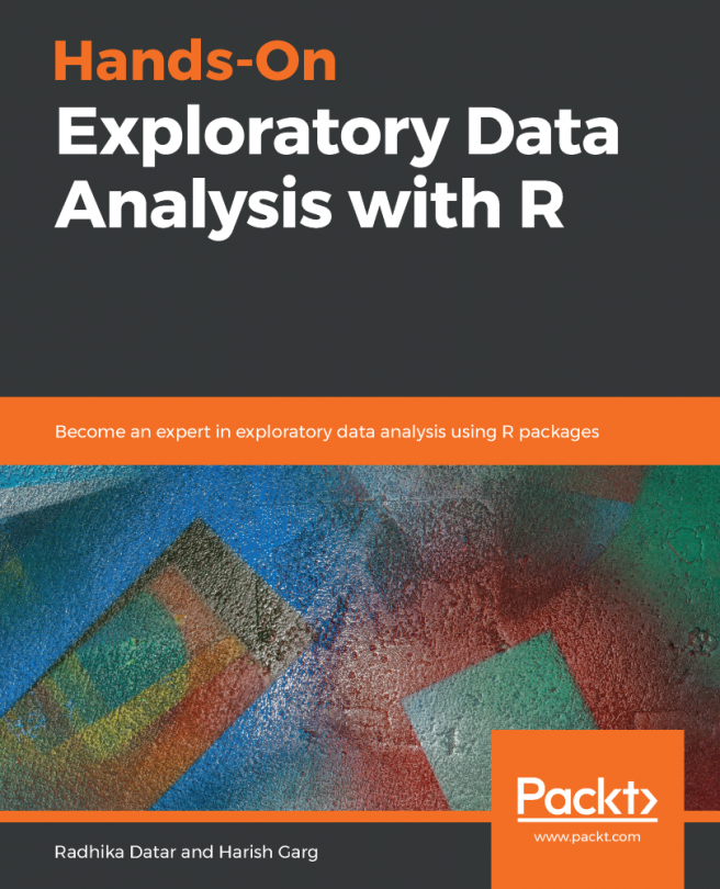
You're reading from  Hands-On Exploratory Data Analysis with R

Product typeBook
Published inMay 2019
Reading LevelIntermediate
PublisherPackt
ISBN-139781789804379
Edition1st Edition
Languages
Tools
Right arrow
Authors (2):
Radhika Datar
Radhika Datar
author image
Radhika Datar

Radhika Datar has more than 5 years' experience in software development and content writing. She is well versed in frameworks such as Python, PHP, and Java, and regularly provides training on them. She has been working with Educba and Eduonix as a training consultant since June 2016, while also working as a freelance academic writer in data science and data analytics. She obtained her master's degree from the Symbiosis Institute of Computer Studies and Research and her bachelor's degree from K. J. Somaiya College of Science and Commerce.
Read more about Radhika Datar

Harish Garg
Harish Garg
author image
Harish Garg

Harish Garg is a Principal Software Developer, author, and co-founder of a software development and training company, Bignumworks. Harish has more than 19 years of experience in a wide variety of technologies, including blockchain, data science and enterprise software. During this time, he has worked for companies such as McAfee, Intel, etc.
Read more about Harish Garg

View More author details
Right arrow

Time Series Datasets

This chapter will introduce a time series dataset and help us to understand how to use EDA techniques to analyze the data. We will also learn about and use EDA techniques using an autocorrelation plot, spectrum plot, complex demodulation amplitude plot, and phase plots. In this chapter, we will first learn how to read and tidy up the data, after which we will learn how to map and understand the underlying structure of the dataset, and identify the important variables. We will then learn how to create a list of outliers or other anomalies using Grubbs' test. We will also cover the parsimonious model and Bartlett's test.

The following topics will be covered in this chapter:

  • Introducing and reading in the data
  • Cleaning and tidying up the data
  • Mapping and understanding the underlying structure of the dataset, and identifying the most important variables...
Technical requirements

You should have hands-on experience or knowledge of the following points before getting started with this chapter:

  • R programming language
  • RStudio
  • R packages (including readr, readxl, jsonlite, httr, rvest, DBI, dplyr, stringr, forcats, lubridate, hms, blob, ggplot2, and knitr)

Introducing and reading the dataset

In this chapter, we will focus on the dataset that consists of the responses of a gas with the help of a multi-sensor device. The dataset includes an hourly response average, which is being recorded along with gas concentrations and proportions. This dataset is referred to as an Air Quality Dataset.

You can download the file from the following link:

https://github.com/PacktPublishing/Hands-On-Exploratory-Data-Analysis-with-R/tree/master/ch07.

For more information, you can refer to the link specified as follows:
https://archive.ics.uci.edu/ml/machine-learning-databases/00360/.

In this section, we will be focusing on reading the attributes of the dataset and converting the .csv or .xls file to a data frame or dataset in the R workspace (with workspace, we are referring to the R environment where various data manipulations can be performed). As...

Cleaning the dataset

Data cleaning, or tidying up the data, is the process of transforming raw data into a specific form of consistent data, which includes analysis in a simple manner. The R programming language includes a set of comprehensive tools that are specifically designed to clean the data in an effective manner. We will be focusing on cleaning the dataset here in a specific way by observing the following steps:

  1. Include the libraries that are required to clean and tidy up the dataset:
> library(dplyr) 
> library(tidyr)

  1. Analyze the summary of our dataset, which will help us to focus on the attributes we need to work on:
> summary(AirQualityUCI) 
      Date                          Time                         CO(GT)         PT08.S1(CO)      NMHC(GT)      
 Min.   :2004-03-10 00:00:00   Min.   :1899-12-31 00:00:00   Min.   :-200.00   Min.   :-200   Min.   ...

Mapping and understanding structure

This section involves understanding each and every attribute in depth, which is considered to be important for the dataset specified.

We need to carry out the following steps to understand the data structure and mapping attributes, if any:

  1. Try to get a feel for the data as per the attribute structure:
> class(AirQualityUCI) 
[1] "tbl_df"     "tbl"        "data.frame" 

The output shows that the dataset is merely a tabular format of a data frame.

  1. Check the dimensions of the dataset:
> dim(AirQualityUCI) 
[1] 9357 15

This shows that the dataset comprises 9357 rows and 15 columns. The column structure has already been discussed in the first section.

  1. View the column names of the dataset. We need to check whether these correspond to the records included in the Excel file:
> colnames(AirQualityUCI) 
[1...

Hypothesis test

This section is all about hypothesis testing in R. This testing is merely an assumption made by the researcher regarding the population of data collected for any experiment. The first step entails an introduction to the statistical hypothesis in R, and later we will cover the decision error in R, which includes one- and two-sample t-tests, u-tests, correlation, and covariance in R.

t-test in R

This is also known as Student's t-test, which is a method for comparing two samples. It can usually be implemented to determine whether the samples are proper or different. This is considered as a parametric test, and the data should be normally distributed. R can handle the various versions of the t-test using the...

Grubbs' test and checking outliers

In R programming, an outlier is merely an observation that is unique in comparison with most of the other observations. An outlier is present because of errors in measurement in the data frame.

The following script is used to detect the particular outliers for each and every attribute:

> outlierKD <- function(dt, var) { 
+     var_name <- eval(substitute(var),eval(dt)) 
+     na1 <- sum(is.na(var_name)) 
+     m1 <- mean(var_name, na.rm = T) 
+     par(mfrow=c(2, 2), oma=c(0,0,3,0)) 
+     boxplot(var_name, main="With outliers") 
+     hist(var_name, main="With outliers", xlab=NA, ylab=NA) 
+     outlier <- boxplot.stats(var_name)$out 
+     mo <- mean(outlier) 
+     var_name <- ifelse(var_name %in% outlier, NA, var_name) 
+     boxplot(var_name, main="Without outliers") 
+     hist...

Parsimonious models

Parsimonious models are simple models with great explanatory predictive power. They usually explain data with a minimum number of parameters, or predictor variables. MoEClust is the R package that fits finite Gaussian mixtures of experts' models. It uses a range of parsimonious covariance with the help of EM or CEM algorithms.

Follow these steps to create a range of parsimonious covariance models with our AirQualityUCI dataset:

  1. Install the package that is required to create a parsimonious model of our dataset:
> install.packages('devtools') 
Installing package into 'C:/Users/Radhika/Documents/R/win-library/3.5' 
(as 'lib' is unspecified) 
trying URL 'https://cran.rstudio.com/bin/windows/contrib/3.5/devtools_2.0.2.zip' 
Content type 'application/zip' length 383720 bytes (374 KB) 
downloaded 374 KB ...

Bartlett's test

Bartlett's test is useful when executing a comparison between two or more samples to specify whether they are taken from populations with equal variance. Bartlett's test works successfully for normally distributed data. This test includes a null hypothesis, with a calculation of equal variances, and the alternative hypothesis, where variances are not considered equal. This test is considered useful for checking the assumptions regarding variance analysis.

The user can perform Bartlett's test with the bartlett.test function in R. The normal syntax for this is as follows :

> bartlett.test(values~groups, dataset)  

Here, the parameters refer to the following:

  • values: The name of the variable containing the data value
  • groups: The name of the variable that specifies which sample each value belongs to

If the data is in an unstacked form (with...

Data visualization

In this section, we will focus on the creation of the following plots:

  • Autocorrelation
  • Spectrum
  • Phase

Autocorrelation plots

Autocorrelation plots are regarded as plots for creating randomness in a particular dataset. This randomness is very powerful regarding autocorrelations of data values with varying time lags. It is mandatory that autocorrelations for any dataset should be near zero, for any and all time-lag separations.

The Acf function computes (and, by default, plots) an estimate of the autocorrelation function of a (possibly multivariate) time series. The syntax is as follows:

> Acf(x, lag.max = NULL, type = c("correlation", "covariance","partial"), plot = TRUE...

Summary

In this chapter, we focused on the implementation of all the libraries of a univariate dataset, which holds a strong representation for time series creation. The best illustration considered in this chapter is the measurement of pollution with respect to parsimonious models with RH and AH. We have listed some of the various packages that are available for reading, in various kinds of attributes, within the dataset indicated in R. There are lots of different options, and even the options we have listed have a wide functionality that we are going to cover and use as we progress through the book.

In the next chapter, we will cover multivariate datasets. Multivariate datasets include a combination of fixed and continuous variables that help us with further exploratory analysis.

lock icon
The rest of the chapter is locked
You have been reading a chapter from
Hands-On Exploratory Data Analysis with R
Published in: May 2019Publisher: PacktISBN-13: 9781789804379
Register for a free Packt account to unlock a world of extra content!
A free Packt account unlocks extra newsletters, articles, discounted offers, and much more. Start advancing your knowledge today.
undefined
Unlock this book and the full library FREE for 7 days
Get unlimited access to 7000+ expert-authored eBooks and videos courses covering every tech area you can think of
Renews at $15.99/month. Cancel anytime

Authors (2)

author image
Radhika Datar

Radhika Datar has more than 5 years' experience in software development and content writing. She is well versed in frameworks such as Python, PHP, and Java, and regularly provides training on them. She has been working with Educba and Eduonix as a training consultant since June 2016, while also working as a freelance academic writer in data science and data analytics. She obtained her master's degree from the Symbiosis Institute of Computer Studies and Research and her bachelor's degree from K. J. Somaiya College of Science and Commerce.
Read more about Radhika Datar

author image
Harish Garg

Harish Garg is a Principal Software Developer, author, and co-founder of a software development and training company, Bignumworks. Harish has more than 19 years of experience in a wide variety of technologies, including blockchain, data science and enterprise software. During this time, he has worked for companies such as McAfee, Intel, etc.
Read more about Harish Garg