Reader small image

You're reading from  Computer Vision Projects with OpenCV and Python 3

Product typeBook
Published inDec 2018
Reading LevelIntermediate
PublisherPackt
ISBN-139781789954555
Edition1st Edition
Languages
Tools
Right arrow
Author (1)
Matthew Rever
Matthew Rever
author image
Matthew Rever

Matthew Rever received his PhD. in electrical engineering from the University of Michigan, Ann Arbor. His career revolves around image processing, computer vision, and machine learning for scientific research applications. He started programming in C++, a language he still uses today, over 20 years ago, and has also used Matlab and most heavily Python in the past few years, using OpenCV, SciPy, scikit-learn, TensorFlow, and PyTorch. He believes it is important to stay up to date on the latest tools to be as productive as possible. Dr. Rever is the author of Packt's Computer Vision Projects with Python 3 and Advanced Computer Vision Projects.
Read more about Matthew Rever

Right arrow

Setting Up an Anaconda Environment

Welcome to Computer Vision Projects with OpenCV and Python 3. This book is one you might want to check out if you're new to OpenCV, and to computer vision in general.

In this chapter, we will be installing all the required tools that we're going to use in the book. We will be dealing with Python 3, OpenCV, and TensorFlow.

You might be wondering: why should I be using Python 3, and not Python 2? The answer to your question is on Python's own website:

"Python 2 is legacy, Python 3 is the present future of the language."

We are looking to the future here, and if we want to future-proof our code, it's better to use Python 3. If you're using Python 2, some of the code examples here might not run, so we'll install Python 3 and use that for all the projects in the book.

In this chapter, we will cover the following topics:

  • Introducing and installing Python and Anaconda
  • Installing the additional libraries
  • Exploring Jupyter Notebook

Introducing and installing Python and Anaconda

The first thing we need is Python 3. The best way to install this is by downloading Continuum Analytics and the Anaconda distribution.

Anaconda is a fully-featured Python distribution that comes with a lot of packages, including numerical analytics, data science, and computer vision. It's going to make our lives a whole lot easier, because it provides us with libraries that are not present in the base Python distribution.

The best part about Anaconda is that it gives us the conda package manager, along with pip, which makes it very easy to install external packages for our Python distribution.

Let's get started.

Installing Anaconda

We will begin by setting up our Anaconda and Python distribution, using the following steps:

  1. Go to the Anaconda website, using the following link www.anaconda.com/download. You should see a landing page that looks similar to the following screenshot:
  1. Next, select your OS and download the latest version of the Anaconda distribution, which includes Python 3.7. Click the Download button, as shown in the following screenshot:
The installer for Windows is graphical; however, you might need to use a command-line installer for macOS or Linux.

Installing the setup file is pretty straightforward, so we won't go through each step here.

  1. When you have everything properly installed and your path variables defined, go to the Command Prompt and make sure everything is good to go by typing the where python command. This shows us all the directories in which Python is installed. You should see something similar to the following screenshot:

As seen in the preceding screenshot, we see that the first instance of Python is in our Anaconda distribution. This means that we can proceed with our Python programs.

In macOS or Linux, the command would be which python instead of where python.
  1. Now, let's make sure we have our other tools. Our first tool will be IPython, which is essentially a command shell for interactive computing in multiple programming languages. We will check it using the where ipython command, as shown in the following screenshot:
  1. The next package we will check is the pip tool, which is the Python installer package. We do this with the where pip command, as shown in the following screenshot:
  1. The next tool to check is the conda package, which is Anaconda's built-in package manager. This is done using the where conda command, as shown in the following screenshot:

We should be good to go with Python now.

If you run which python on macOS or Linux, and it says something such as user/bin/Python, that means Python is either not installed or it's not the first thing in our path, so we should modify that as per our system.

In the next section, we're going to cover installing additional libraries such as OpenCV, TensorFlow, dlib, and Tesseract, which will be used for the projects in this book.

Installing additional libraries

All the packages that we will be installing in this section are vital for our upcoming projects. So, let's get started.

Installing OpenCV

To get OpenCV, go to the following link: anaconda.org/conda-forge/opencv. Technically, we don't need to access the website to install this package. The site just shows the various versions of OpenCV and all the different systems we can install it on.

Copy and paste the installation command from the site into Command Prompt and then run it, as shown in the following screenshot:

The preceding command is a simple, platform-independent way to get OpenCV. There are other methods for getting it; however, using this command ensures that we are installing the latest version.

Installing dlib

We need to install dlib from the Anaconda distribution, similar to OpenCV. Just as with OpenCV, installing dlib is a straightforward process.

Run the following command:

conda install -c menpo dlib

You will get the following output:

This will take around 10 to 20 seconds to run. If everything goes well, we should be good to go with dlib.

Installing Tesseract

Tesseract is Google's optical character recognition library, and is not natively a Python package. Because of this, there's a Python binding for it that calls the executable, which can then be installed manually.

Go to the GitHub repository for Tesseract, which is found at the following link: https://github.com/tesseract-ocr/tesseract.

Scroll down to the Installing Tesseract section in the GitHub readme. Here, we are presented with two options:

  • Installing it via a pre-built binary package
  • Building it from source

We want to install it via the pre-built binary package, so click on that link. We can also build it from source if we want to, but that doesn't really offer any advantages. The Tesseract Wiki explains the steps to install it on various different operating systems.

As we're using Windows, and we want to install a pre-built one, click on the Tesseract at UB Mannheim link, where you will find all the latest setup files. Download the latest setup from the site.

Once downloaded, run the installer or execute the command. However, this is not going to put Tesseract in your path. We need to make sure it is in your path; otherwise, when you call Tesseract from within Python, you're going to get an error message.

So, we need to figure out where Tesseract is and modify our path variable. To do this, type the where tesseract command in Command Prompt, as shown in the following screenshot:

Once you have the binary packages, use the pip command to apply the Python binding to the packages. Use the following commands:

$ pip install tesseract
$ pip install pytesseract

We should be good to go with Tesseract now.

Installing TensorFlow

Last but not least, we will install TensorFlow, which is a software library for data flow programming across a range of tasks. It is usually used for machine learning applications such as neural networks.

To install it, go to TensorFlow's website at the following link: tensorflow.org/install/. The website contains instructions for all the major operating systems.

As we're using Windows, the installation process is very simple. We just have to run the pip install tensorflow command in Command Prompt, as seen in the following screenshot:

As seen in the preceding screenshot, TensorFlow is already installed on the system, so it says that the requirements are satisfied. We should be good to go with TensorFlow now.

Install tensorflow-hub using the following command:

pip install tensorflow-hub

Next, install tflearn using the following command:

pip install tflearn

Finally, Keras is a high-level interface, which can be installed using the following command:

pip install keras

We have installed OpenCV, TensorFlow, dlib, and Tesseract, so we should be good to go with the tools for our book. Our next step will be exploring Jupyter Notebook, which should be fun!

Exploring Jupyter Notebook

Now that we have our libraries installed, we're ready to get started with Jupyter Notebook. Jupyter Notebook is a really nice way of creating interactive code and widgets. It lets us create interactive presentations with live code and experiment, as we're doing here.

If everything is set up correctly using Anaconda, we should already have Jupyter installed. Let's go ahead and take a look at Jupyter Notebook now.

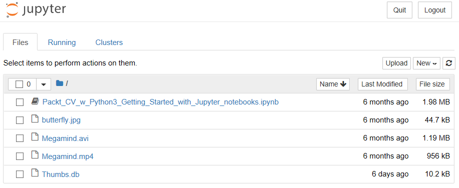
Open Command Prompt in the directory where your code files are, and then run the jupyter notebook command. This will open up a web browser in the directory where the command was executed. This should result in an interface that looks similar to the following screenshot:

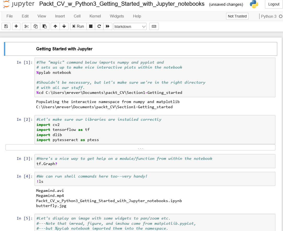
Next, open the .ipynb file so you can explore the basic functionalities of Jupyter Notebook. Once opened, we should see a page similar to the following screenshot:

As shown, there are blocks (called cells) where we can put in Python commands and Python code. We can also enter other commands, also known as magic commands, which are not part of Python per se, but allow us to do nice things within Jupyter or IPython (an interactive shell for Python). The % at the beginning means that the command is a magic command.

The biggest advantage here is that we can execute individual lines of code, instead of having to type out the entire code block in one go.

If you're new to Jupyter Notebook, go to the following link: https://www.cheatography.com/weidadeyue/cheat-sheets/jupyter-notebook/. Here, they list Jupyter Notebook keyboard shortcuts, which can be really useful for quick code testing.

Let's go through some of the commands seen in the preceding screenshot, and see what they do, as follows:

  1. The %pylab notebook command, as seen in the first cell, imports a lot of very useful and common libraries, particularly NumPy and PyPlot, without us needing to explicitly call the import commands. It also sets up a Notebook easily.
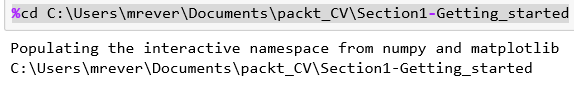
  2. Also in the first cell, we assign the directory that we will be working from, as follows:
%cd C:\Users\<user_name>\Documents\<Folder_name>\Section1-Getting_started

This results in the following output:

So far, so good!

  1. The following cell shows how to import our libraries. We're going to import OpenCV, TensorFlow, dlib, and Tesseract, just to make sure that everything is working and that there aren't any nasty surprises. This is done using the following code block:
import cv2
import tensorflow as tf
import dlib
import pytesseract as ptess

If you get an error message here, redo the installation of the libraries, following the instructions carefully. Sometimes things do go wrong, depending on our system.

  1. The third cell in the screenshot contains the command for importing the graph module in TensorFlow. This can come in handy for getting help on a function from within the Notebook, as follows:
tf.Graph?

We will discuss this function in Chapter 7, Deep Learning Image Classification with TensorFlow.

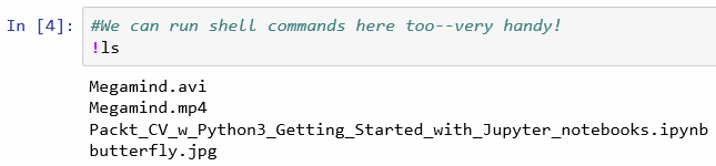
  1. Another neat thing about Jupyter Notebooks is that we can run shell commands right in the cell. As seen in the fourth cell in the screenshot (repeated here), the ls command shows us all the files in the directory we are working from:
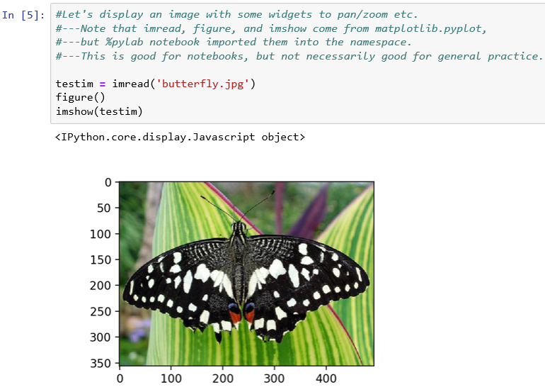
  1. In this book, we'll be working with a lot of images, so we'll want to see the images right in the Notebook. Use the imread() function to read the image file from your directory. After that, your next step is to create a figure() widget to display the image. Finally, use the imshow() function to actually display the image.

This entire process is summarized in the following screenshot:

This is awesome, because we have widgets that are flexible.

  1. By grabbing the bottom-right corner, we can shrink this to a reasonable size to see our color image with pixel axes displayed. We also have the pan option available. By clicking on it, we can pan our image and box zoom it. Hitting the home button resets the original view.

We will want take a look at our images, and processed images and so forth—as seen previously, this is a very handy and simple way to do it. We can also use PyLab inline, which is useful for certain things, as we'll see.

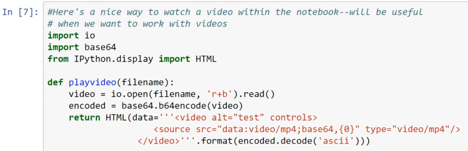
  1. As we know, part of computer vision is working with videos. To play videos within the notebook, we need to import some libraries and use IPython's HTML capability, as shown in the following screenshot:

Essentially, we're using our web browser's capability to play back videos. So, it's not really Python that's doing it, but our web browser, which enables interactivity between Jupyter Notebook and our browser.

Here, we defined the playvideo() function, which takes the video filename as an input and returns an HTML object with our video.

  1. Execute the following command on Jupyter to play the Megamind video. It's just a clip of the movie Megamind, which (for some reason) comes with OpenCV if we download all the source code:
playvideo(' ./Megamind.mp4')
  1. You will see a black box, and if you scroll down, you'll find a play button. Hit this and the movie will play, as seen in the following screenshot:

This can be used to play our own videos. All you have to do is point the command to the video that you want to play.

Once you have all this running, you should be in good shape to run the projects that we're going to take a look at in the coming chapters.

Summary

In this chapter, we learned about the Anaconda distribution and different ways to install Python. We learned how to set up Python using the Anaconda distribution.

Next, we looked at how to install various libraries in Anaconda, to make it easier for us to run various programs. Finally, we learned the basics of Jupyter Notebook and how it works.

In the next chapter, Chapter 2, Image Captioning with TensorFlow, we will look at how to carry out image captioning using TensorFlow.

You have been reading a chapter from
Computer Vision Projects with OpenCV and Python 3
Published in: Dec 2018Publisher: PacktISBN-13: 9781789954555
Register for a free Packt account to unlock a world of extra content!
A free Packt account unlocks extra newsletters, articles, discounted offers, and much more. Start advancing your knowledge today.
undefined
Unlock this book and the full library FREE for 7 days
Get unlimited access to 7000+ expert-authored eBooks and videos courses covering every tech area you can think of
Renews at $15.99/month. Cancel anytime

Author (1)

author image
Matthew Rever

Matthew Rever received his PhD. in electrical engineering from the University of Michigan, Ann Arbor. His career revolves around image processing, computer vision, and machine learning for scientific research applications. He started programming in C++, a language he still uses today, over 20 years ago, and has also used Matlab and most heavily Python in the past few years, using OpenCV, SciPy, scikit-learn, TensorFlow, and PyTorch. He believes it is important to stay up to date on the latest tools to be as productive as possible. Dr. Rever is the author of Packt's Computer Vision Projects with Python 3 and Advanced Computer Vision Projects.
Read more about Matthew Rever