Reader small image

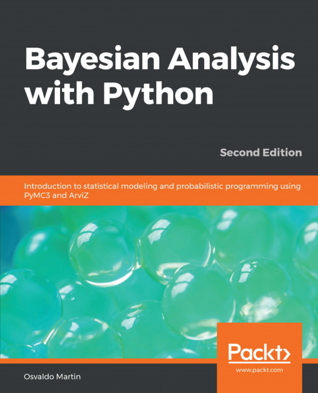
You're reading from  Bayesian Analysis with Python. - Second Edition

Product typeBook
Published inDec 2018
Reading LevelIntermediate
PublisherPackt
ISBN-139781789341652
Edition2nd Edition
Languages
Concepts
Right arrow
Author (1)
Osvaldo Martin
Osvaldo Martin
author image
Osvaldo Martin

Osvaldo Martin is a researcher at CONICET, in Argentina. He has experience using Markov Chain Monte Carlo methods to simulate molecules and perform Bayesian inference. He loves to use Python to solve data analysis problems. He is especially motivated by the development and implementation of software tools for Bayesian statistics and probabilistic modeling. He is an open-source developer, and he contributes to Python libraries like PyMC, ArviZ and Bambi among others. He is interested in all aspects of the Bayesian workflow, including numerical methods for inference, diagnosis of sampling, evaluation and criticism of models, comparison of models and presentation of results.
Read more about Osvaldo Martin

Right arrow

Generalizing Linear Models

We think in generalities, but we live in detail.
- Alfred North Whitehead

In the last chapter, we used a linear combination of input variables to predict the mean of an output variable. We assumed the latter to be distributed as a Gaussian. Using a Gaussian works in many situations, but for many other it could be wiser to choose a different distribution; we already saw an example of this when we replaced the Gaussian distribution with a Student's t-distribution. In this chapter, we will see more examples where it is wise to use distributions other than Gaussian. As we will learn, there is a general motif, or pattern, that can be used to generalize the linear model to many problems.

In this chapter, we will explore:

  • Generalized linear models
  • Logistic regression and inverse link functions
  • Simple logistic regression
  • Multiple logistic regression
  • ...

Generalized linear models

One of the core ideas of this chapter is rather simple: in order to predict the mean of an output variable, we can apply an arbitrary function to a linear combination of input variable.

Where is a function, we will call inverse link function. There are many inverse link functions we can choose; probably the simplest one is the identity function. This is a function that returns the same value used as its argument. All models from Chapter 3, Modeling with Linear Regression used the identity function, and for simplicity we just omit it. The identity function may not be very useful on its own, but it allows us to think of several different models in a more unified way.

Why do we call f, the inverse link function, instead of just the link function? Because traditionally people apply functions to the other side of equation 4.1, and unfortunately for us,...

Logistic regression

Regression problems are about predicting a continuous value for an output variable given the values of one or more input variables. Instead, classification is about assigning a discrete value (representing a discrete class) to an output variable given some input variables. In both cases, the task is to get a model that properly models the mapping between output and input variables; in order to do so, we have at our disposal a sample with correct pairs of output-input variables. From a machine learning perspective, both regressions and classifications are instances of supervised learning algorithms.

My mother prepares a delicious dish called sopa seca, which is basically a spaghetti-based recipe and literally means dry soup. While it may sound like a misnomer or even an oxymoron, the name of the dish makes total sense when we learn how it is cooked. Something...

Multiple logistic regression

In a similar fashion to multiple linear regression, multiple logistic regression is about using more than one independent variable. Let's try combining the sepal length and the sepal width. Remember we need to pre-process the data a little bit:

df = iris.query("species == ('setosa', 'versicolor')") 
y_1 = pd.Categorical(df['species']).codes
x_n = ['sepal_length', 'sepal_width']
x_1 = df[x_n].values

The boundary decision

Feel free to skip this section and jump to the model implementation (next section) if you are not too interested in how we can derive the boundary decision.

From the model, we have the following equation:

And from...

Poisson regression

Another very popular generalized linear model is the Poisson regression. This model assumes data is distributed according to the, wait for it... Poisson distribution.

One scenario where Poisson distribution is useful is when counting things, such as the decay of a radioactive nucleus, the number of children per couple, or the number of Twitter followers. What all these examples have in common is that we usually model them using discrete non-negative numbers: {0, 1, 2, 3, ....}. This type of variable receives the name of count data.

Poisson distribution

Imagine we are counting the number of red cars passing through an avenue per hour. We could use Poisson distribution to describe this data. Poisson distribution...

Robust logistic regression

We just saw how to fix an excess of zeros without directly modeling the factor that generates them. A similar approach, suggested by Kruschke, can be used to perform a more robust version of logistic regression. Remember that in logistic regression, we model the data as binomial, that is, zeros and ones. So it may happen that we find a dataset with unusual zeros and/or ones. Take, as an example, the iris dataset that we already saw, but with some added intruders:

iris = sns.load_dataset("iris") 
df = iris.query("species == ('setosa', 'versicolor')")
y_0 = pd.Categorical(df['species']).codes
x_n = 'sepal_length'
x_0 = df[x_n].values
y_0 = np.concatenate((y_0, np.ones(6, dtype=int)))
x_0 = np.concatenate((x_0, [4.2, 4.5, 4.0, 4.3, 4.2, 4.4]))
x_c = x_0 - x_0.mean()
plt.plot(x_c, y_0, 'o&apos...

The GLM module

As we discussed at the beginning of this chapter, linear models are very useful statistical tools. Extensions such as the ones we saw in this chapter make them even more general tools. For that reason, PyMC3 includes a module to simplify the creation of linear models: the Generalized Liner Model (GLM) module. For example, a simple linear regression will be as follows:

with pm.Model() as model: 
    glm.glm('y ~ x', data) 
    trace = sample(2000) 

The second line of the preceding code takes care of adding priors for the intercept and for the slope. By default, the intercept is assigned a flat prior, and the slopes an prior. Note that the maximum a posteriori (MAP) of the default model will be essentially equivalent to the one obtained using the ordinary least squared method. These is totally fine as a default linear regression; you can change it using...

Summary

The main idea discussed in this chapter is a rather simple one: in order to predict the mean of an output variable, we can apply an arbitrary function to a linear combination of input variables. I know I already said this at the beginning of the chapter, but repetition is important. We call that arbitrary function the inverse link function. The only restriction we have in choosing such a function is that the output has to be adequate to be used as a parameter of the sampling distribution (generally the mean). One situation in which we would like to use an inverse link function is when working with categorical variables, another is when the data can only take positive values, and yet another is when we need a variable in the [0, 1] interval. All these different variations become different models; many of those models are routinely used as statistical tools, and their application...

Exercises

  1. Rerun the first model using the petal length and then petal width variables. What are the main differences in the results? How wide or narrow is the 95% HPD interval in each case?
  2. Repeat exercise 1, this time using a Student's t-distribution as a weakly informative prior. Try different values of .
  3. Go back to the first example, the logistic regression for classifying setosa or versicolor given sepal length. Try to solve the same problem using a simple linear regression model, as we saw in Chapter 3, Modeling with Linear Regression. How useful is linear regression compared to logistic regression? Can the result be interpreted as a probability? Tip, check whether the values of are restricted to the [0, 1] interval.
  1. In the example from the Interpreting the coefficients of a logistic regression section, we changed sepal_length by 1 unit. Using Figure 4.6, corroborate...
lock icon
The rest of the chapter is locked
You have been reading a chapter from
Bayesian Analysis with Python. - Second Edition
Published in: Dec 2018Publisher: PacktISBN-13: 9781789341652
Register for a free Packt account to unlock a world of extra content!
A free Packt account unlocks extra newsletters, articles, discounted offers, and much more. Start advancing your knowledge today.
undefined
Unlock this book and the full library FREE for 7 days
Get unlimited access to 7000+ expert-authored eBooks and videos courses covering every tech area you can think of
Renews at $15.99/month. Cancel anytime

Author (1)

author image
Osvaldo Martin

Osvaldo Martin is a researcher at CONICET, in Argentina. He has experience using Markov Chain Monte Carlo methods to simulate molecules and perform Bayesian inference. He loves to use Python to solve data analysis problems. He is especially motivated by the development and implementation of software tools for Bayesian statistics and probabilistic modeling. He is an open-source developer, and he contributes to Python libraries like PyMC, ArviZ and Bambi among others. He is interested in all aspects of the Bayesian workflow, including numerical methods for inference, diagnosis of sampling, evaluation and criticism of models, comparison of models and presentation of results.
Read more about Osvaldo Martin