Using the tikzpicture environment

In the previous chapter, we saw that we basically load TikZ and then use a tikzpicture environment that contains our drawing commands. Let’s go step by step to create a document that will be the base of all our drawings in this chapter. Our goal is to draw a rectangular grid with dotted lines. Such a grid is really beneficial in positioning objects in our pictures later on. I usually start with such a helper grid, make my drawing, and take the grid out in the final version of the drawing.

As it’s one of our first TikZ examples, we will do it step by step and then discuss how it works:

1. Open your LaTeX editor. Start with the standalone document class. In the class options, use the tikz option and define a border of 10 pt:

   \documentclass[tikz,border=10pt]{standalone}

2. Begin the document environment:

   \begin{document}

3. Next, begin a tikzpicture environment:

   \begin{tikzpicture}

4. Draw a thin, dotted grid from the coordinate (-3,-3) to the coordinate (3,3):

   \draw[thin,dotted] (-3,-3) grid (3,3);

5. To better see where the horizontal and vertical axis is, let’s draw them with an arrow tip:

   \draw[->] (-3,0) -- (3,0);

   \draw[->] (0,-3) -- (0,3);

6. End the tikzpicture environment:

   \end{tikzpicture}

7. End the document:

   \end{document}

Compile the document and look at the output:

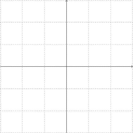
Figure 2.1 – A rectangular grid

In step 1, we used the standalone document class. That class allows us to create documents that consist only of a single drawing and cuts the PDF document to the actual content. Therefore, we don’t have an A4 or letter page with just a tiny drawing, plus a lot of white space and margins.

To get a small margin of 10 pt around the picture, we wrote border=10pt because, with a small margin, it looks nicer in a PDF viewer. Since the standalone class is designed for drawings, it provides a tikz option. As we set that option, the class loads TikZ automatically, so we don’t have to add \usepackage{tikz} anymore.

After we started the document in step 1, we opened a tikzpicture environment in step 3. Every drawing command will happen in this environment until we end it. As it’s a LaTeX environment, it can be used with optional arguments. For example, we could write \begin{tikzpicture}[color=red] to get everything we draw in red unless we specify otherwise. We will talk about valuable options later in this book.

Step 4 was our main task of drawing a grid. We used the \draw command that we will see exceptionally often throughout this book. We specified the following:

• How: We added thin and dotted options in square brackets because that’s the LaTeX syntax for optional arguments. So, everything the \draw command does will now be in thin and dotted lines.
• Where: We set (-3,-3) as the start coordinate and (3,3) as the end coordinate. We will look thoroughly at the coordinates in the next section.
• What: The grid element is like a rectangle where one corner is the start coordinate, to the left of it, and the other corner is the end coordinate, to the right of it. It fills this rectangle with a grid of lines. They are, as we required before, thin and dotted.

\draw produces a path with coordinates and picture elements in between until we end with a semicolon. We can sketch it like the following:

\draw[<style>] <coordinate> <picture element> <coordinate> ... ;

Every path must end with a semicolon. Paths with coordinates, elements, and options can be pretty complex and flexible – the rule to end paths with a semicolon allows TikZ to parse and understand where such paths end and other commands follow.

The lines in a grid have a distance of 1 by default. The optional step argument can change that. For example, you could write grid[step=0.5] or do that right at the beginning as the \draw option, such as the following:

\draw[thin,dotted,step=0.5] <coordinate>
  <picture element> <coordinate> ... ;

In step 5, we have drawn two lines. The picture element here is a straight line between the coordinates given. We use the convenient -- shortcut that stands for a line. The -> style determines that we shall have an arrow tip at the end. In the next section, we will draw many lines.

Finally, we just ended the tikzpicture and document environments.

TikZ, document classes, and figures

In this book, we will focus on TikZ picture creation. Remember that we can use TikZ with any LaTeX class, such as article, book, or report. Furthermore, TikZ pictures can be used in a figure environment with label and caption, just like \includegraphics.

While this section showed a manageable number of commands, we should have a closer look at the concept of coordinates, which is now the topic of our next section.