

1.5 Applications to financial services
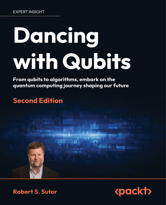
Suppose we have a circle of radius 1 inscribed in a square, as in Figure 1.12. The sides of the square have length 2, and the square’s area is 4 = 2 × 2. What is the area A of the circle?
Before you try to remember your geometric area formulas, let’s compute the area of a circle using ratios and some experiments.
Suppose we drop some number N of coins onto the square and count how many have their centers on or inside the circle. If C is this number, then

A ≈ 4C/N.
There is randomness involved here: it’s possible they all land inside the circle or, less likely, outside the circle. For N = 1, we do not get an accurate estimate of A because C/N can only be 0 or 1.
Exercise 1.3
If N = 2, what are the possible estimates of A? What about if N = 3?
We will get a better estimate for A if we choose N large.
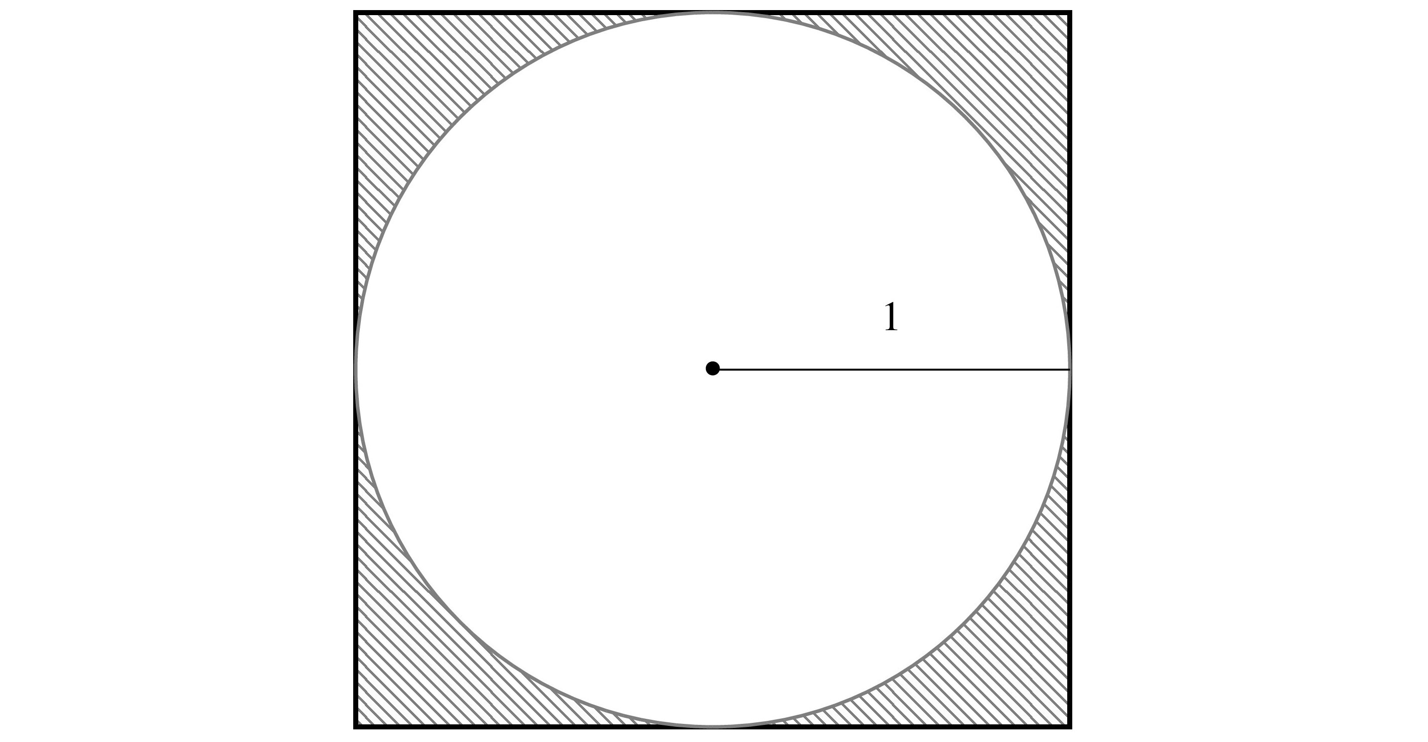
I created 10 points whose centers lie inside the square using Python and its random number generator. The plot in Figure 1.13 shows where they landed. In this case, C = 9, and so A ≈ 3.6.
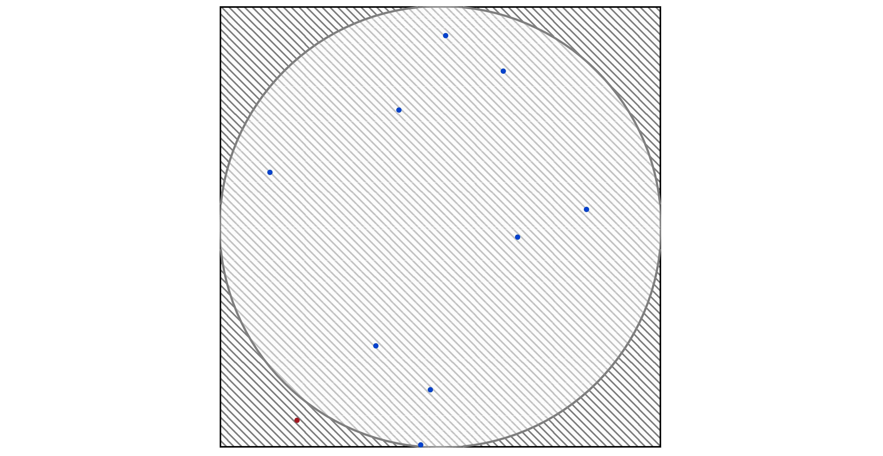
For N = 100, we get a more interesting plot in Figure 1.14 with C = 84 and A ≈ 3.36. Remember, this value would be different if I had generated other random numbers.
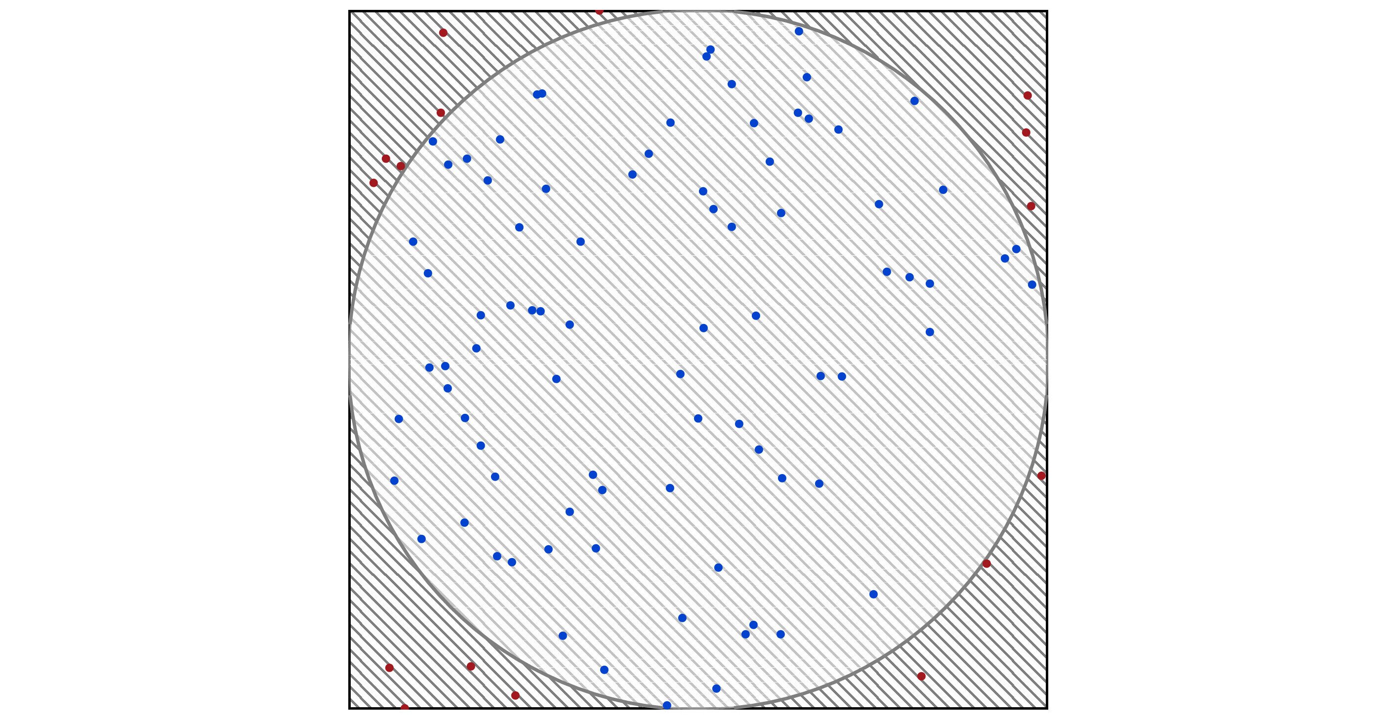
The final plot is in Figure 1.15 for N = 500. Now C = 387 and A ≈ 3.096.
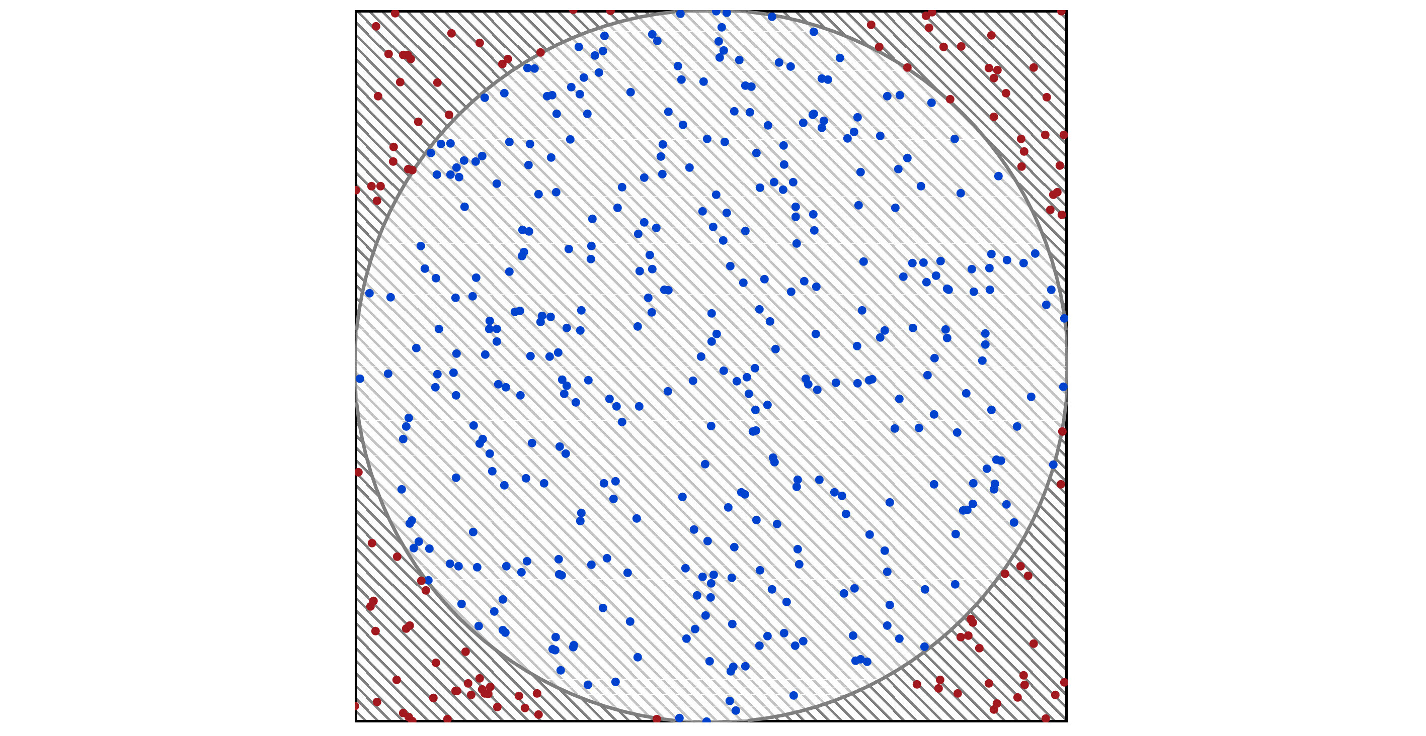
The real value of A is π ≈ 3.1415926. We call this technique Monte Carlo sampling, which goes back to the 1940s. algorithm$Monte Carlo Monte Carlo algorithm
Using the same technique, here are approximations of A for increasingly large N. Remember, we are using random numbers, so these numbers will vary based on the sequence of values used.

That’s a lot of runs, the value of N, to get close to the actual value of π. Nevertheless, this example demonstrates how we can use Monte Carlo sampling techniques to approximate the value of something when we may not have a formula. In this case, we estimated A. For the example, we ignored our knowledge that the formula for the area of a circle is π r2, where r is the circle’s radius.
In section 6.8, we work through the math and show that if we want to estimate π within 0.00001 with a probability of at least 99.9999%, we need N ≥ 82863028. We need to use more than 82 million points! So it is possible to use a Monte Carlo method here, but it is not efficient.
In this example, we know the answer ahead of time by other means. Monte Carlo methods can be a useful tool if we do not know the answer and do not have a nice neat formula to compute. However, the very large number of samples needed to get decent accuracy makes the process computationally intensive. If we can reduce the sample count significantly, we can compute a more accurate result much faster.
Given that the title of this section mentions “finance,” I now note, perhaps unsurprisingly, that quantitative analysts use Monte Carlo methods in computational finance. financial services
The randomness we employ to calculate π translates over into ideas such as uncertainties. Uncertainties can then be related to probabilities, which we use to calculate the risk and rate of return of investments.
Instead of looking at whether a point is inside or outside a circle, for the rate of return, we might consider several factors that go into calculating the risk. For example,
- market size
- share of the market
- selling price
- fixed costs
- operating costs
- obsolescence
- inflation or deflation
- national monetary policy
- weather
- political factors and election results
For each of these or any other factor relevant to the particular investment, we quantify them and assign probabilities to the possible results. In a weighted way, we combine all possible combinations to compute risk. This is a function that we cannot calculate all at once, but we can use Monte Carlo methods to estimate. Techniques similar to, but more complicated than, the circle analysis in section 6.8, give us how many samples we need to use to get a result within the desired accuracy.
In the circle example, reasonable accuracy can require tens of millions of samples. We might need many orders of magnitude greater for an investment risk analysis. So what do we do?
We can and do use High-Performance Computers (HPC). We can consider fewer possibilities for each factor. For example, we might vary the possible selling prices by larger amounts. We can consult better experts and get more accurate probabilities. This could improve the result but not necessarily the computation time. Or, we can take fewer samples and accept less precise results. HPC
Alternatively, we could consider quantum variations and replacements for Monte Carlo methods. In 2015, Ashley Montanaro 152 described a quadratic speedup using quantum computers. How much improvement does this give us? Instead of the 82 million samples required for the circle calculation with the above accuracy, we could do it in something closer to 9,000 samples (9055 ≈ √82000000). Montanaro, Ashley
In 2019, Stamatopoulos et al. showed methods and considerations for pricing financial options using quantum computing systems. 206
I want to stress that to do this, we need much larger, more accurate, and more powerful quantum computers than we have at the time of writing. However, like much of the algorithmic work researchers are doing on industry use cases, I believe we are getting on the right path to solve significant problems significantly faster using quantum computation.
By using Monte Carlo methods, we can vary our assumptions and do scenario analysis. If we can eventually use quantum computers to significantly reduce the number of samples, we can look at far more scenarios much faster.
To learn more
David Hertz’ original 1964 paper in the Harvard Business Review is a very readable introduction to Monte Carlo methods for risk analysis without ever using the phrase “Monte Carlo.” 110 A more recent paper gives more of the history of these methods and applies them to marketing analytics. 87
My goal with this book is to give you enough of an introduction to quantum computing so that you can read industry-specific quantum use cases and research papers. For example, to learn about modern quantum algorithmic approaches to risk analysis, see the articles by Woerner, Egger, et al. 237 76 Some early results on heuristics using quantum computation for transaction settlements are covered in Braine et al. 23