Reader small image

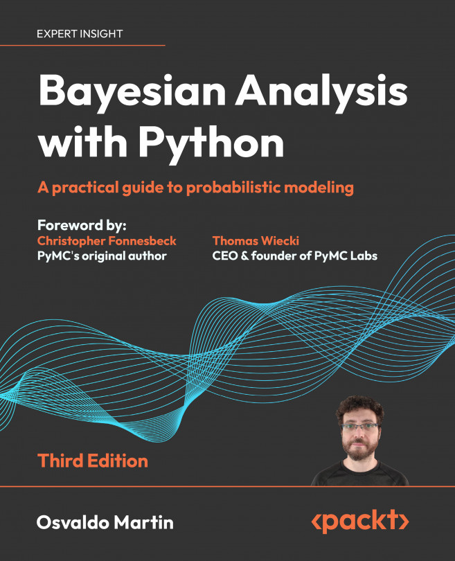
You're reading from  Bayesian Analysis with Python - Third Edition

Product typeBook
Published inJan 2024
Reading LevelExpert
PublisherPackt
ISBN-139781805127161
Edition3rd Edition
Languages
Right arrow
Author (1)
Osvaldo Martin
Osvaldo Martin
author image
Osvaldo Martin

Osvaldo Martin is a researcher at CONICET, in Argentina. He has experience using Markov Chain Monte Carlo methods to simulate molecules and perform Bayesian inference. He loves to use Python to solve data analysis problems. He is especially motivated by the development and implementation of software tools for Bayesian statistics and probabilistic modeling. He is an open-source developer, and he contributes to Python libraries like PyMC, ArviZ and Bambi among others. He is interested in all aspects of the Bayesian workflow, including numerical methods for inference, diagnosis of sampling, evaluation and criticism of models, comparison of models and presentation of results.
Read more about Osvaldo Martin

Right arrow

Chapter 7
Mixture Models

...the father has the form of a lion, the mother of an ant; the father eats flesh and the mother herbs. And these breed the ant-lion... –The Book of Imaginary Beings

The River Plate (also known as La Plata River or Río de la Plata) is the widest river on Earth and a natural border between Argentina and Uruguay. During the late 19th century, the port area along this river was a place where indigenous people mixed with Africans (most of them slaves) and European immigrants. One consequence of this encounter was the mix of European music, such as the waltz and mazurka, with the African candombe and Argentinian milonga (which, in turn, is a mix of Afro-American rhythms), giving origin to the dance and music we now call the tango.

Mixing previously existing elements is a great way to create new things, not only in the context of music. In statistics, mixture models are one common approach to model building. These models are built by mixing simpler...
7.1 Understanding mixture models

Mixture models naturally arise when the overall population is a combination of distinct sub-populations. A familiar example is the distribution of heights in a given adult human population, which can be described as a mixture of female and male sub-populations. Another classical example is the clustering of handwritten digits. In this case, it is very reasonable to expect 10 sub-populations, at least in a base 10 system! If we know to which sub-population each observation belongs, it is generally a good idea to use that information to model each sub-population as a separate group. However, when we do not have direct access to this information, mixture models come in handy.

Blends of Distributions

Many datasets cannot be properly described using a single probability distribution, but they can be described as a mixture of such distributions. Models that assume data comes from a mixture of distributions are known as mixture models.

When building a...

7.2 Finite mixture models

One way to build mixture models is to consider a finite weighted mixture of two or more distributions. Then the probability density of the observed data is a weighted sum of the probability density of K subgroups:

 ∑K p(y) = wip (y | θi) i=1

We can interpret wi as the probability of the component i, and thus its values are restricted to the interval [0, 1] and they need to sum up to 1. The components p(y|θi) are usually simple distributions, such as a Gaussian or a Poisson. If K is finite, we have a finite mixture model. To fit such a model, we need to provide a value of K, either because we know the correct value beforehand or because we can make an educated guess.

Conceptually, to solve a mixture model, all we need to do is properly assign each data point to one of the components. In a probabilistic model, we can do this by introducing a random variable, whose function is to specify to which component a particular observation is assigned. This variable is generally referred...

7.3 The non-identifiability of mixture models

The means parameter has shape 2, and from Figure 7.6 we can see that one of its values is around 47 and the other is close to 57.5. The funny thing is that we have one chain saying that means[0] is 47 and the other 3 saying it is 57.5, and the opposite for mmeans[1]. Thus, if we compute the mean of mmeans[0], we will get some value close to 55 (57.5 × 3 + 47 × 1), which is not the correct value. What we are seeing is an example of a phenomenon known as parameter non-identifiability. This happens because, from the perspective of the model, there is no difference if component 1 has a mean of 47 and component 2 has a mean of 57.5 or vice versa; both scenarios are equivalent. In the context of mixture models, this is also known as the label-switching problem.

Non-Identifiability

A statistical model is non-identifiable if one or more of its parameters cannot be uniquely determined. Parameters in a model are not identified if the...

7.4 How to choose K

One of the main concerns with finite mixture models is how to decide on the number of components. A rule of thumb is to begin with a relatively small number of components and then increase it to improve the model-fit evaluation. As we already know from Chapter 5, model fit can be evaluated using posterior-predictive checks, metrics such as the ELPD, and the expertise of the modeler(s).

Let us compare the model for K = {2,3,4,5}. To do this, we are going to fit the model four times and then save the data and model objects for later use:

Code 7.4

Ks = [2, 3, 4, 5] 
 
models = [] 
idatas = [] 
for k in Ks: 
    with pm.Model() as model: 
        p = pm.Dirichlet('p', a=np.ones(k)) 
        means = pm.Normal('means', 
               ...

7.5 Zero-Inflated and hurdle models

When counting things, like cars on a road, stars in the sky, moles on your skin, or virtually anything else, one option is to not count a thing, that is, to get zero. The number zero can generally occur for many reasons; we get a zero because we were counting red cars and a red car did not go down the street or because we missed it. If we use a Poisson or NegativeBinomial distribution to model such data, we will notice that the model generates fewer zeros compared to the data. How do we fix that? We may try to address the exact cause of our model predicting fewer zeros than the observed and include that factor in the model. But, as is often the case, it may be enough, and simpler, to assume that we have a mixture of two processes:

  • One modeled by a discrete distribution with probability

  • One giving extra zeros with probability 1

In some texts, you will find that represents the extra zeros instead of 1 . This is not a big deal;...

7.6 Mixture models and clustering

Clustering or cluster analysis is the data analysis task of grouping objects in such a way that objects in a given group are closer to each other than to those in the other groups. The groups are called clusters and the degree of closeness can be computed in many different ways, for example, by using metrics, such as the Euclidean distance. If instead we take the probabilistic route, then a mixture model arises as a natural candidate to solve clustering tasks.

Performing clustering using probabilistic models is usually known as model-based clustering. Using a probabilistic model allows us to compute the probability of each data point belonging to each one of the clusters. This is known as soft clustering instead of hard clustering, where each data point belongs to a cluster with a probability of 0 or 1. We can turn soft clustering into hard clustering by introducing some rule or boundary. In fact, you may remember that this is exactly what we do to...

7.7 Non-finite mixture model

For some problems, such as trying to cluster handwritten digits, it is easy to justify the number of groups we expect to find in the data. For other problems, we can have good guesses; for example, we may know that our sample of Iris flowers was taken from a region where only three species of Iris grow, thus using three components is a reasonable starting point. When we are not that sure about the number of components, we can use model selection to help us choose the number of groups. Nevertheless, for other problems, choosing the number of groups a priori can be a shortcoming, or we may instead be interested in estimating this number directly from the data. A Bayesian solution for this type of problem is related to the Dirichlet process.

7.7.1 Dirichlet process

All the models that we have seen so far have been parametric models, meaning models with a fixed number of parameters that we are interested in estimating, like a fixed number of clusters. We...

7.8 Continuous mixtures

The focus of this chapter was on discrete mixture models, but we can also have continuous mixture models. And indeed we already know some of them. For instance, hierarchical models can also be interpreted as continuous mixture models where the parameters in each group come from a continuous distribution in the upper level. To make it more concrete, think about performing linear regression for several groups. We can assume that each group has its own slope or that all the groups share the same slope. Alternatively, instead of framing our problem as two extreme discrete options, a hierarchical model allows us to effectively model a continuous mixture of these two options.

7.8.1 Some common distributions are mixtures

The BetaBinomial is a discrete distribution generally used to describe the number of successes y for n Bernoulli trials when the probability of success p at each trial is unknown and assumed to follow a beta distribution with parameters α and...

7.9 Summary

Many problems can be described as an overall population composed of distinct sub-populations. When we know to which sub-population each observation belongs, we can specifically model each sub-population as a separate group. However, many times we do not have direct access to this information, thus it may be appropriate to model that data using mixture models. We can use mixture models to try to capture true sub-populations in the data or as a general statistical trick to model complex distributions by combining simpler distributions.

In this chapter, we divided mixture models into three classes: finite mixture models, non-finite mixture models, and continuous mixture models. A finite mixture model is a finite weighted mixture of two or more distributions, each distribution or component representing a subgroup of the data. In principle, the components can be virtually anything we may consider useful from simple distributions, such as a Gaussian or a Poisson, to more complex...

7.10 Exercises

  1. Generate synthetic data from a mixture of 3 Gaussians. Check the accompanying Jupyter notebook for this chapter for an example of how to do this. Fit a finite Gaussian mixture model with 2, 3, or 4 components.

  2. Use LOO to compare the results from exercise 1.

  3. Read and run through the following examples about mixture models from the PyMC documentation:

  4. Refit fish_data using a NegativeBinomial and a Hurdle NegativeBinomial model. Use rootograms to compare these two models with the Zero-Inflated Poisson model shown in this chapter.

  5. Repeat exercise 1 using a Dirichlet process.

  6. Assuming for a moment that you do not know the correct species/labels for the iris dataset, use a mixture model to cluster the...

Join our community Discord space

Join our Discord community to meet like-minded people and learn alongside more than 5000 members at: https://packt.link/bayesian

PIC

lock icon
The rest of the chapter is locked
You have been reading a chapter from
Bayesian Analysis with Python - Third Edition
Published in: Jan 2024Publisher: PacktISBN-13: 9781805127161
Register for a free Packt account to unlock a world of extra content!
A free Packt account unlocks extra newsletters, articles, discounted offers, and much more. Start advancing your knowledge today.
undefined
Unlock this book and the full library FREE for 7 days
Get unlimited access to 7000+ expert-authored eBooks and videos courses covering every tech area you can think of
Renews at £13.99/month. Cancel anytime

Author (1)

author image
Osvaldo Martin

Osvaldo Martin is a researcher at CONICET, in Argentina. He has experience using Markov Chain Monte Carlo methods to simulate molecules and perform Bayesian inference. He loves to use Python to solve data analysis problems. He is especially motivated by the development and implementation of software tools for Bayesian statistics and probabilistic modeling. He is an open-source developer, and he contributes to Python libraries like PyMC, ArviZ and Bambi among others. He is interested in all aspects of the Bayesian workflow, including numerical methods for inference, diagnosis of sampling, evaluation and criticism of models, comparison of models and presentation of results.
Read more about Osvaldo Martin