Learning Objectives

By the end of this chapter, you will be able to:

• Explain data and its types
• Classify data based on its characteristics
• Calculate basic univariate statistics about data
• Identify outliers
• Use bivariate analysis to understand the relationship between two variables

In this chapter, we will cover the basics of data analytics and statistics. You will also learn how to identify outliers and gain an understanding of the relationship between variables.

Data has fundamentally transformed the 21st century. Thanks to easy access to computers, companies and organizations have been able to change the way they work with larger and more complex datasets. Using data, insights that would have been virtually impossible to find 50 years ago can now be found with just a few lines of computer code. In this chapter, we will discuss what data is and how data analysis can be used to unlock insights and recognize patterns.

Let's start with the first question: what is data? Data (the plural of the word datum) can be thought of as recorded measurements of something in the real world. For example, a list of heights is data – that is, height is a measure of the distance between a person's head and their feet. We usually call that something the data is describing a unit of observation. In the case of these heights, a person is the unit of observation.

As you can imagine, there is a lot of data that we can gather to describe a person – including their age, weight, whether they are a smoker, and more. One or more of these measurements used to describe one specific unit of observation is called a data point, and each measurement in a data point is called a variable (this is also often referred to as a feature). When you have several data points together, you have a dataset.

Types of Data

Data can also be broken down into two main categories: quantitative and qualitative:

Figure 1.1: The classification of types of data

Quantitative data is a measurement that can be described as a number; qualitative data is data that is described by non-numerical values, such as text. Your height is data that would be described as quantitative. However, describing yourself as either a "smoker" or a "non-smoker" would be considered qualitative data.

Quantitative data can be further classified into two subcategories: discrete and continuous. Discrete quantitative values are values that can take on a fixed level of precision – usually integers. For example, the number of surgeries you have had in your life is a discrete value – you can have 0, 1, or more surgeries, but you cannot have 1.5 surgeries. A continuous variable is a value that, in theory, could be divided with an arbitrary amount of precision. For example, your body mass could be described with arbitrary precision to be 55, 55.3, 55.32, and so on. In practice, of course, measuring instruments limit our precision. However, if a value could be described with higher precision, then it is generally considered continuous.

Note

Qualitative data can generally be converted into quantitative data, and quantitative data can also be converted into qualitative data. This is explained later in the chapter using an example.

Let's think about this using the example of being a "smoker" versus a "non-smoker". While you can describe yourself to be in the category of "smoker" or "non-smoker", you could also reimagine these categories as answers to the statement "you smoke regularly", and then use the Boolean values of 0 and 1 to represent "true" and "false," respectively.

Similarly, in the opposite direction, quantitative data, such as height, can be converted into qualitative data. For example, instead of thinking of an adult's height as a number in inches or centimeters (cm), you can classify them into groups, with people greater than 72 inches (that is, 183 cm) in the category "tall," people between 63 inches and 72 inches (that is, between 160 and 183 cm) as "medium," and people shorter than 63 inches (that is, 152 cm) as "short."

Data Analytics and Statistics

Raw data, by itself, is simply a group of values. However, it is not very interesting in this form. It is only when we start to find patterns in the data and begin to interpret them that we can start to do interesting things such as make predictions about the future and identify unexpected changes. These patterns in the data are referred to as information. Eventually, a large organized collection of persistent and extensive information and experience that can be used to describe and predict phenomena in the real world is called knowledge. Data analysis is the process by which we convert data into information and, thereafter, knowledge. When data analysis is combined with making predictions, we then have data analytics.

There are a lot of tools that are available to make sense of data. One of the most powerful tools in the toolbox of data analysis is using mathematics on datasets. One of these mathematical tools is statistics.

Types of Statistics

Statistics can be further divided into two subcategories: descriptive statistics and inferential statistics.

Descriptive statistics are used to describe data. Descriptive statistics on a single variable in a dataset are referred to as univariate analysis, while descriptive statistics that look at two or more variables at the same time are referred to as multivariate analysis.

In contrast, inferential statistics think of datasets as a sample, or a small portion of measurements from a larger group called a population. For example, a survey of 10,000 voters in a national election is a sample of the entire population of voters in a country. Inferential statistics are used to try to infer the properties of a population, based on the properties of a sample.

Note

In this book, we will primarily be focusing on descriptive statistics. For more information on inferential statistics, please refer to a statistics textbook, such as Statistics, by David Freedman, Robert Pisani, and Roger Purves.

Example:

Imagine that you are a health policy analyst and are given the following dataset with information about patients:

Figure 1.2: Healthcare data

When given a dataset, it's often helpful to classify the underlying data. In this case, the unit of observation for the dataset is an individual patient, because each row represents an individual observation, which is a unique patient. There are 10 data points, each with 5 variables. Three of the columns, Year of Birth, Height, and Number of Doctor Visits, are quantitative because they are represented by numbers. Two of the columns, Eye Color and Country of Birth, are qualitative.

Activity 1: Classifying a New Dataset

In this activity, we will classify the data in a dataset. You are about to start a job in a new city at an up-and-coming start-up. You're excited to start your new job, but you've decided to sell all your belongings before you head off. This includes your car. You're not sure at what price to sell it for, so you decide to collect some data. You ask some friends and family who recently sold their cars what the make of the car was, and how much they sold the cars for. Based on this information, you now have a dataset.

The data is as follows:

Figure 1.3: Used car sales data

Steps to follow:

1. Determine the unit of observation.
2. Classify the three columns as either quantitative or qualitative.
3. Convert the Make column into quantitative data columns.

   Note

   The solution for this activity can be found via this link.

As previously mentioned, descriptive statistics is one of the ways in which we can analyze data in order to understand it. Both univariate and multivariate analysis can give us an insight into what might be going on with a phenomenon. In this section, we will take a closer look at the basic mathematical techniques that we can use to better understand and describe a dataset.

Univariate Analysis

As previously mentioned, one of the main branches of statistics is univariate analysis. These methods are used to understand a single variable in a dataset. In this section, we will look at some of the most common univariate analysis techniques.

Data Frequency Distribution

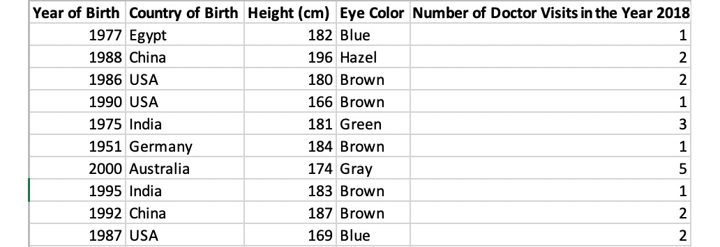
The distribution of data is simply a count of the number of values that are in a dataset. For example, let's say that we have a dataset of 1,000 medical records, and one of the variables in the dataset is eye color. If we look at the dataset and find that 700 people have brown eyes, 200 people have green eyes, and 100 people have blue eyes, then we have just described the distribution of the dataset. Specifically, we have described the absolute frequency distribution. If we were to describe the counts not by the actual number of occurrences in the dataset, but as the proportion of the total number of data points, then we are describing its relative frequency distribution. In the preceding eye color example, the relative frequency distribution would be 70% brown eyes, 20% green eyes, and 10% blue eyes.

It's easy to calculate a distribution when the variable can take on a small number of fixed values such as eye color. But what about a quantitative variable that can take on many different values, such as height? The general way to calculate distributions for these types of variables is to make interval "buckets" that these values can be assigned to and then calculate distributions using these buckets. For example, height can be broken down into 5-cm interval buckets to make the following absolute distribution (please refer to Figure 1.6). We can then divide each row in the table by the total number of data points (that is, 10,000) and get the relative distribution.

Another useful thing to do with distributions is to graph them. We will now create a histogram, which is a graphical representation of the continuous distribution using interval buckets.

Exercise 1: Creating a Histogram

In this exercise, we will use Microsoft Excel to create a histogram. Imagine, as a healthcare policy analyst, that you want to see the distribution of heights to note any patterns. To accomplish this task, we need to create a histogram.

Note

We can use spreadsheet software such as Excel, Python, or R to create histograms. For convenience, we will use Excel. Also, all the datasets used in this chapter, can be found on GitHub: https://github.com/TrainingByPackt/SQL-for-Data-Analytics/tree/master/Datasets.

Perform the following steps:

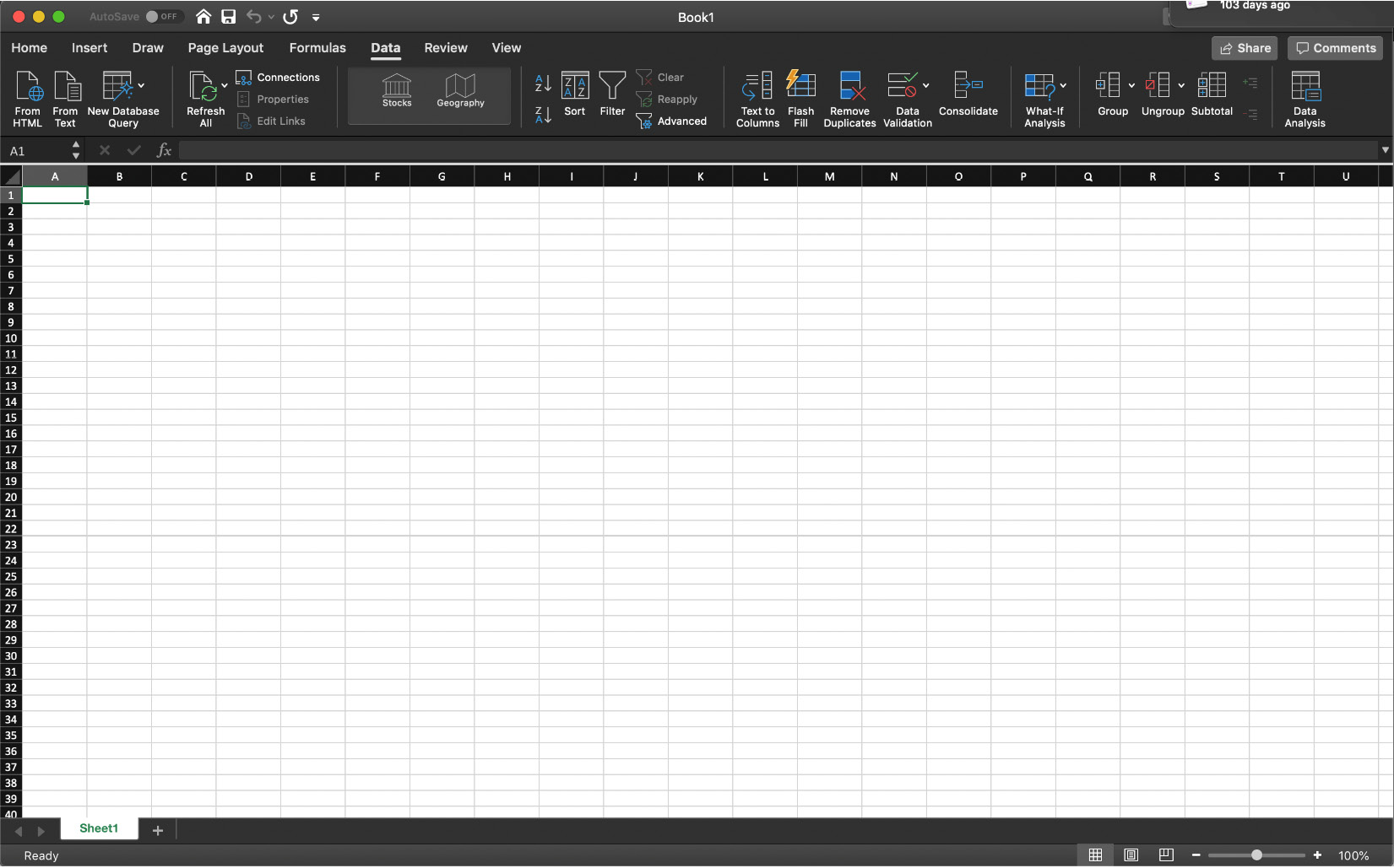
1. Open Microsoft Excel to a blank workbook:
   

   Figure 1.4: A blank Excel workbook

2. Go to the Data tab and click on From Text.
3. You can find the heights.csv dataset file in the Datasets folder of the GitHub repository. After navigating to it, click on OK.
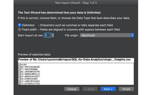
4. Choose the Delimited option in the Text Import Wizard dialog box, and make sure that you start the import at row 1. Now, click on Next:
   

   Figure 1.5: Selecting the Delimited option

5. Select the delimiter for your file. As this file is only one column, it has no delimiters, although CSVs traditionally use commas as delimiters (in future, use whatever is appropriate for your dataset). Now, click on Next.
6. Select General for the Column Data Format. Now, click on Finish.
7. For the dialog box asking Where you want to put the data?, select Existing Sheet, and leave what is in the textbox next to it as is. Now, click on OK.
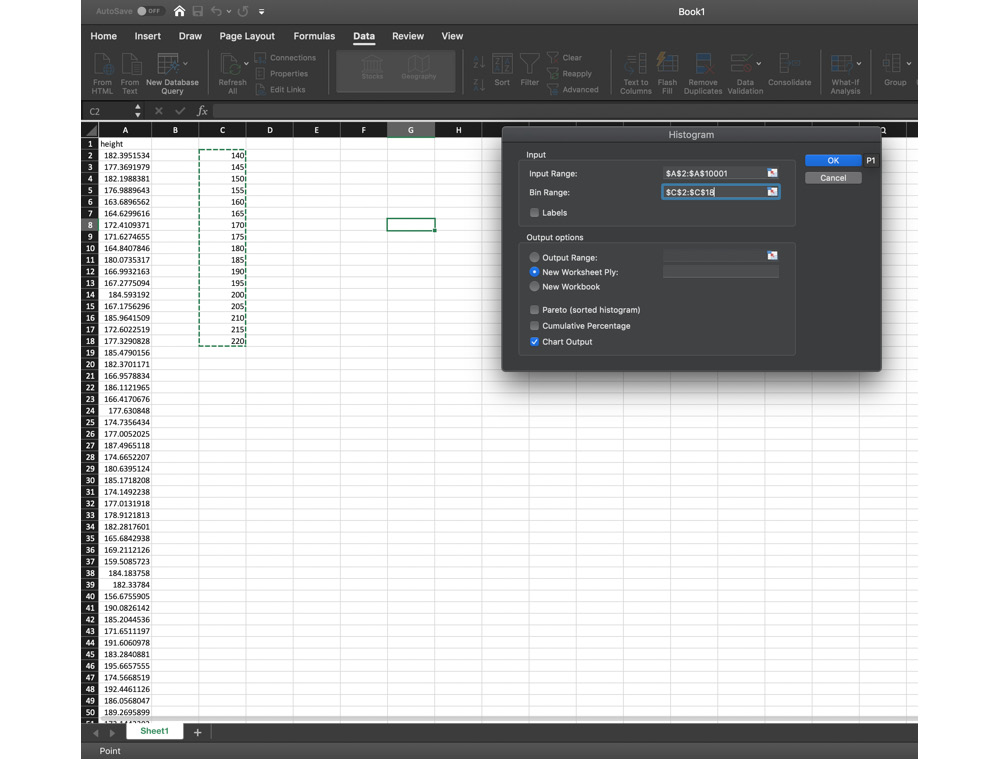
8. In column C, write the numbers 140, 145, and 150 in increments of 5 all the way to 220 in cells C2 to C18, as seen in Figure 1.6:
   

   Figure 1.6: Entering the data into the Excel sheet

9. Under the Data tab, click on Data Analysis (if you don't see the Data Analysis tab, follow these instructions to install it: https://support.office.com/en-us/article/load-the-analysis-toolpak-in-excel-6a63e598-cd6d-42e3-9317-6b40ba1a66b4).
10. From the selection box that pops up, select Histogram. Now, click on OK.
11. For Input Range, click on the selection button in the far-right side of the textbox. You should be returned to the Sheet1 worksheet, along with a blank box with a button that has a red arrow in it. Drag and highlight all the data in Sheet1 from A2 to A10001. Now, click on the arrow with the red button.
12. For Bin Range, click on the selection button in the far-right side of the textbox. You should be returned to the Sheet1 worksheet, along with a blank box with a button that has a red arrow in it. Drag and highlight all the data in Sheet1 from C2 to C18. Now, click on the arrow with the red button.
13. Under Output Options, select New Worksheet Ply, and make sure Chart Output is marked, as seen in Figure 1.7. Now, click on OK:
    

    Figure 1.7: Selecting New Worksheet Ply

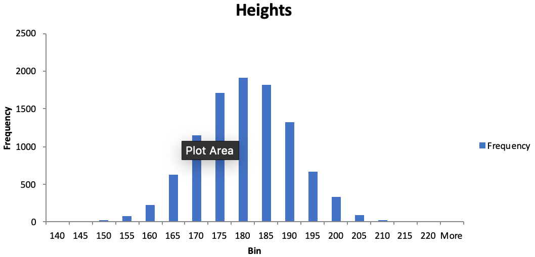
14. Click on Sheet2. Find the graph and double-click on the title where it says Histogram. Type the word Heights. You should produce a graph that is similar to the one in the following diagram:

Figure 1.8: Height distribution for adult males

Looking at the shape of the distribution can help you to find interesting patterns. Notice here the symmetric bell-shaped curl of this distribution. This distribution is often found in many datasets and is known as the normal distribution. This book won't go into too much detail about this distribution but keep an eye out for it in your data analysis – it shows up quite often.

Quantiles

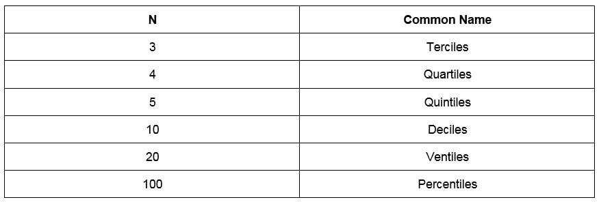
One way to quantify data distribution numerically is to use quantiles. N-quantiles are a set of n-1 points used to divide a variable into n groups. These points are often called cut points. For example, a 4-quantile (also referred to as quartiles) is a group of three points that divide a variable into four, approximately equal groups of numbers. There are several common names for quantiles that are used interchangeably, and these are as follows:

Figure 1.9: Common names for n-quantiles

The procedure for calculating quantiles actually varies from place to place. We will use the following procedure to calculate the n-quantiles for d data points for a single variable:

1. Order the data points from lowest to highest.
2. Determine the number n of n-quantiles you want to calculate and the number of cut points, n-1.
3. Determine what number k cut point you want to calculate, that is, a number from 1 to n-1. If you are starting the calculation, set k equal to 1.
4. Find the index, i, for the k-th cut point using the following equation:
   

   Figure 1.10: The index

5. If i calculated in number 3 is a whole number, simply pick that numbered item from the ordered data points. If the k-th cut point is not a whole number, find the numbered item that is lower than i, and the one after it. Multiply the difference between the numbered item and the one after it, and then multiply by the decimal portion of the index. Add this number to the lowest numbered item.
6. Repeat Steps 2 to 5 with different values of k until you have calculated all the cut points.

These steps are a little complicated to understand by themselves, so let's work through an exercise. With most modern tools, including SQL, computers can quickly calculate quantiles with built-in functionality.

Exercise 2: Calculating the Quartiles for Add-on Sales

Before you start your new job, your new boss wants you to look at some data before you start on Monday, so that you have a better sense of one of the problems you will be working on – that is, the increasing sales of add-ons and upgrades for car purchases. Your boss sends over a list of 11 car purchases and how much they have spent on add-ons and upgrades to the base model of the new ZoomZoom Model Chi. In this exercise, we will classify the data and calculate the quartiles for the car purchase using Excel. The following are the values of Add-on Sales ($): 5,000, 1,700, 8,200, 1,500, 3,300, 9,000, 2,000, 0, 0, 2,300, and 4,700.

Note

All the datasets used in this chapter, can be found on GitHub: https://github.com/TrainingByPackt/SQL-for-Data-Analytics/tree/master/Datasets.

Perform the following steps to complete the exercise:

1. Open Microsoft Excel to a blank workbook.
2. Go to the Data tab and click on From Text.
3. You can find the auto_upgrades.csv dataset file in the Datasets folder of the GitHub repository. Navigate to the file and click on OK.
4. Choose the Delimited option in the Text Import Wizard dialog box, and make sure to start the import at row 1. Now, click on Next.
5. Select the delimiter for your file. As this file is only one column, it has no delimiters, although CSVs traditionally use commas as delimiters (in future, use whatever is appropriate for your dataset). Now, click on Next.
6. Select General for the Column Data Format. Now, click on Finish.
7. For the dialog box asking Where do you want to put the data?, select Existing Sheet, and leave what is in the textbox next to it as is. Now, click on OK.
8. Click on cell A1. Then, click on the Data tab, and then click on Sort from the tab.
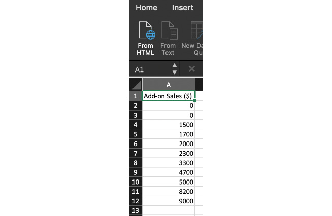
9. A sorted dialog box will pop up. Now, click on OK. The values will now be sorted from lowest to highest. The list in Figure 1.11 shows the sorted values:
   

   Figure 1.11: The Add-on Sales figures sorted

10. Now, determine the number of n-quantiles and cut points you need to calculate. Quartiles are equivalent to 4-tiles, as seen in Figure 1.9. Because the number of cut points is just 1 less than the number of n-quantiles, we know there will be 3 cut points.
11. Calculate the index for the first cut point. In this case, k=1; d, the number of data points, equals 10; and n, the number of n-quantiles, equals 4. Plugging this into the equation from Figure 1.12, we get 3.5:
12. Because index 3.5 is a non-integer, we first find the third and fourth items, which are 1,500 and 1,700, respectively. We find the difference between them, which is 200, and then multiply this by the decimal portion of 0.5, yielding 100. We add this to the third numbered item, 1,500, and get 1,600.
13. Repeat Steps 2 to 5 for k=2 and k=4 to calculate the second and third quartiles. You should get 2,300 and 4,850, respectively.

Figure 1.12: Calculating the index for the first cut point

In this exercise, we learned how to classify the data and calculate the quartiles using Excel.

Central Tendency

One of the common questions asked of a variable in a dataset is what a typical value for that variable is. This value is often described as the central tendency of the variable. There are many numbers calculated from a dataset that are often used to describe its central tendency, each with their own advantages and disadvantages. Some of the ways to measure central tendency include the following:

• Mode: The mode is simply the value that comes up most often in the distribution of a variable. In Figure 1.2, the eye color example, the mode would be "brown eyes," because it occurs the most often in the dataset. If multiple values are tied for the most common variable, then the variable is called multimodal and all of the highest values are reported. If no value is repeated, then there is no mode for those sets of values. Mode tends to be useful when a variable can take on a small, fixed number of values. However, it is problematic to calculate when a variable is a continuous quantitative variable, such as in our height problem. With these variables, other calculations are more appropriate for determining the central tendency.
• Average/Mean: The average of a variable (also called the mean) is the value calculated when you take the sum of all values of the variable and divide by the number of data points. For example, let's say you had a small dataset of ages: 26, 25, 31, 35, and 29. The average of these ages would be 29.2, because that is the number you get when you sum the 5 numbers and then divide by 5, that is, the number of data points. The mean is easy to calculate, and generally does a good job of describing a "typical" value for a variable. No wonder it is one of the most commonly reported descriptive statistics in literature. The average as a central tendency, however, suffers from one major drawback – it is sensitive to outliers. Outliers are data that are significantly different in value from the rest of the data and occur very rarely. Outliers can often be identified by using graphical techniques (such as scatterplots and box plots) and identifying any data points that are very far from the rest of the data. When a dataset has an outlier, it is called a skewed dataset. Some common reasons why outliers occur include unclean data, extremely rare events, and problems with measurement instruments. Outliers often skew the average to a point when they are no longer representative of a typical value in the data.
• Median: The median (also called the second quartile and the fiftieth percentile) is sort of a strange measure of central tendency, but has some serious advantages compared with average. To calculate median, take the numbers for a variable and sort from the lowest to the highest, and then determine the middle number. For an odd number of data points, this number is simply the middle value of the ordered data. If there are an even number of data points, then take the average of the two middle numbers.

  While the median is a bit unwieldy to calculate, it is less affected by outliers, unlike mean. To illustrate this fact, we will calculate the median of the skewed age dataset of 26, 25, 31, 35, 29, and 82. This time, when we calculate the median of the dataset, we get the value of 30. This value is much closer to the typical value of the dataset than the average of 38. This robustness toward outliers is one of the major 'reasons why a median is calculated.

  As a general rule, it is a good idea to calculate both the mean and median of a variable. If there is a significant difference in the value of the mean and the median, then the dataset may have outliers.

Exercise 3: Calculating the Central Tendency of Add-on Sales

In this exercise, we will calculate the central tendency of the given data. To better understand the Add-on Sales data, you will need to gain an understanding of what the typical value for this variable is. We will calculate the mode, mean, and median of the Add-on Sales data. Here is the data for the 11 cars purchased: 5,000, 1,700, 8,200, 1,500, 3,300, 9,000, 2,000, 0, 0, 2,300, and 4,700.

Perform the following steps to implement the exercise:

1. To calculate the mode, find the most common value. Because 0 is the most common value in the dataset, the mode is 0.
2. To calculate the mean, sum the numbers in Add-on Sales, which should equal 37,700. Then, divide the sum by the number of values, 11, and you get the mean of 3,427.27.
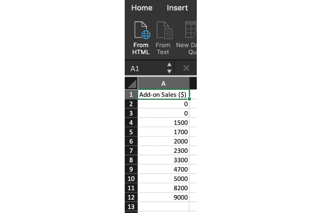
3. Finally, calculate the median by sorting the data, as shown in Figure 1.13:

Figure 1.13: Add-on Sales figures sorted

Determine the middle value. Because there are 11 values, the middle value will be sixth in the list. We now take the sixth element in the ordered data and get a median of 2,300.

Note

When we compare the mean and the median, we see that there is a significant difference between the two. As previously mentioned, it is a sign that we have outliers in our dataset. We will discuss in future sections how to determine which values are outliers.

Dispersion

Another property that is of interest in a dataset is discovering how close together data points are in a variable. For example, the number sets [100, 100, 100] and [50, 100, 150] both have a mean of 100, but the numbers in the second group are spread out more than the first. This property of describing how the data is spread is called dispersion.

There are many ways to measure the dispersion of a variable. Here are some of the most common ways to evaluate dispersion:

• Range: The range is simply the difference between the highest and lowest values for a variable. It is incredibly easy to calculate but is very susceptible to outliers. It also does not provide much information about the spread of values in the middle of the dataset.
• Standard Deviation/Variance: Standard deviation is simply the square root of the average of the squared difference between each data point and the mean. The value of standard deviation ranges from 0 all the way to positive infinity. The closer the standard deviation is to 0, the less the numbers in the dataset vary. If the standard deviation is 0, this means that all the values for a dataset variable are the same.

  One subtle distinction to note is that there are two different formulas for standard deviation, which are shown in Figure 1.14. When the dataset represents the entire population, you should calculate the population standard deviation using formula A in Figure 1.14. If your sample represents a portion of the observations, then you should use formula B for the sample standard deviation, as displayed in Figure 1.14. When in doubt, use the sample variance, as it is considered more conservative. Also, in practice, the difference between the two formulas is very small when there are many data points.

  The standard deviation is generally the quantity used most often to describe dispersion. However, like range, it can also be affected by outliers, though not as extremely as the range is. It can also be fairly involved to calculate. Modern tools, however, usually make it very easy to calculate the standard deviation.

  One final note is that, occasionally, you may see a related value, variance, listed as well. This quantity is simply the square of the standard deviation:

Figure 1.14: The standard deviation formulas for A) population and B) sample

• Interquartile Range (IQR): The interquartile range is the difference between the first quartile, Q1 (this is also called the lower quartile), and the third quartile, Q3 (this is also called the upper quartile).

  Note

  For more information on calculating quantiles and quartiles, refer to the Data Distribution section in this chapter.

IQR, unlike range and standard deviation, is robust toward outliers, and so, while it is the most complicated of the functions to calculate, it provides a more robust way to measure the spread of datasets. In fact, IQR is often used to define outliers. If a value in a dataset is smaller than Q1 - 1.5 X IQR, or larger than Q3 + 1.5 X IQR, then the value is considered an outlier.

Exercise 4: Dispersion of Add-on Sales

To better understand the sales of additions and upgrades, you need to take a closer look at the dispersion of the data. In this exercise, we will calculate the range, standard deviation, IQR, and outliers of Add-on Sales. Here is the data for the 11 cars purchased: 5,000, 1,700, 8,200, 1,500, 3,300, 9,000, 2,000, 0, 0, 2,300, and 4,700.

Follow these steps to perform the exercise:

1. To calculate the range, we find the minimum value of the data, 0, and subtract it from the maximum value of the data, 9,000, yielding 9,000.
2. The standard deviation calculation requires you to do the following: Determine whether we want to calculate the sample standard deviation or the population standard deviation. As these 11 data points only represent a small portion of all purchases, we will calculate the sample standard deviation.
3. Next, find the mean of the dataset, which we calculated in Exercise 2, Calculating the Quartiles for Add-on Sales, to be 3,427.27.
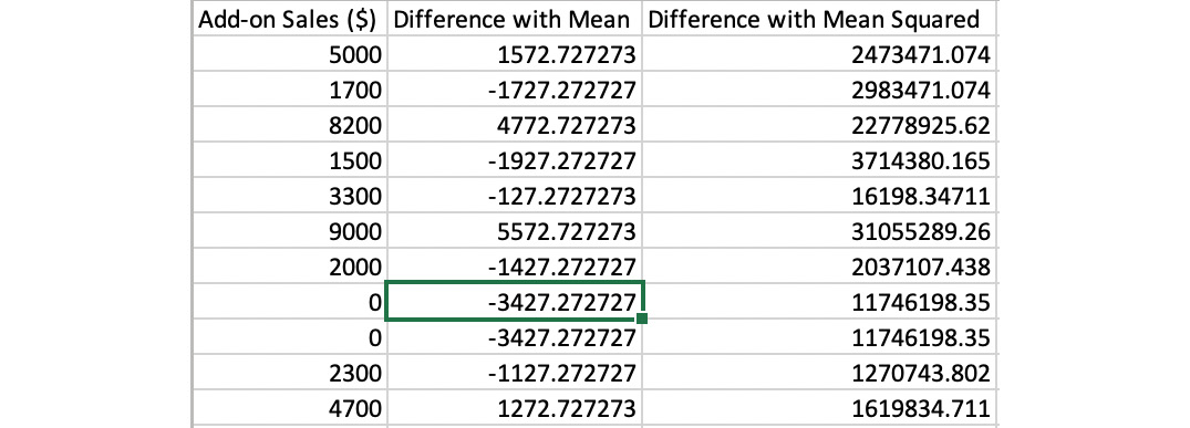
4. Now, subtract each data point from the mean and square the result. The results are summarized in the following diagram:
   

   Figure 1.15: The sum of the calculation of the square

5. Sum up the Differences with Mean Squared values, yielding 91,441,818.
6. Divide the sum by the number of data points minus 1, which, in this case, is 10, and take its square root. This calculation should result in 3,023.93 as the sample standard deviation.
7. To calculate the IQR, find the first and third quartiles. This calculation can be found in Exercise 2, Calculating the Quartiles for Add-on Sales, to give you 1,600 and 4,850. Then, subtract the two to get the value 3,250.

Bivariate Analysis

So far, we have talked about methods for describing a single variable. Now, we will discuss how to find patterns with two variables using bivariate analysis.

Scatterplots

A general principle you will find in analytics is that graphs are incredibly helpful in finding patterns. Just as histograms can help you to understand a single variable, scatterplots can help you to understand two variables. Scatterplots can be produced pretty easily using your favorite spreadsheet.

Note

Scatterplots are particularly helpful when there are only a small number of points, usually some number between 30 and 500. If you have a large number of points and plotting them appears to produce a giant blob in your scatterplot, take a random sample of 200 of those points and then plot them to help discern any interesting trends.

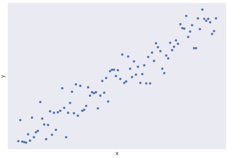
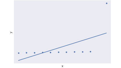
A lot of different patterns are worth looking out for within a scatterplot. The most common pattern people look for is an upward or downward trend between the two variables; that is, as one variable increases, does the other variable decrease? Such a trend indicates that there may be a predictable mathematical relationship between the two variables. Figure 1.16 shows an example of a linear trend:

Figure 1.16: The upward linear trend of two variables, x and y

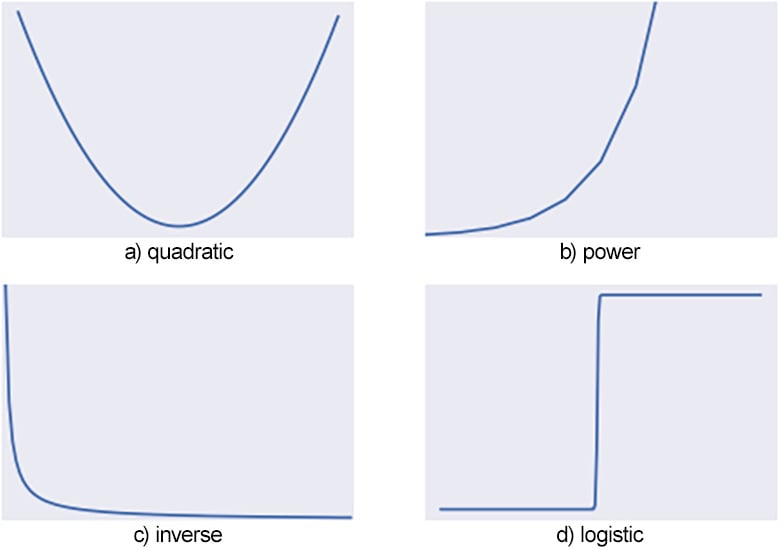
There are also many trends that are worth looking out for that are not linear, including quadratic, exponential, inverse, and logistic. The following diagram shows some of these trends and what they look like:

Figure 1.17: Other common trends

Note

The process of approximating a trend with a mathematical function is known as regression analysis. Regression analysis plays a critical part in analytics but is outside the scope of this book. For more information on regression analysis, refer to an advanced text, such as Regression Modeling Strategies: With Applications to Linear Models, Logistic Regression, and Survival Analysis by Frank E. Harrell Jr.

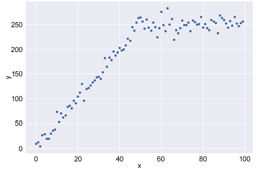
While trends are useful for understanding and predicting patterns, detecting changes in trends are often more important. Changes in trends usually indicate a critical change in whatever you are measuring and are worth examining further for an explanation. The following diagram shows an example of a change in a trend, where the linear trend wears off after x=40:

Figure 1.18: An example of a change in trend

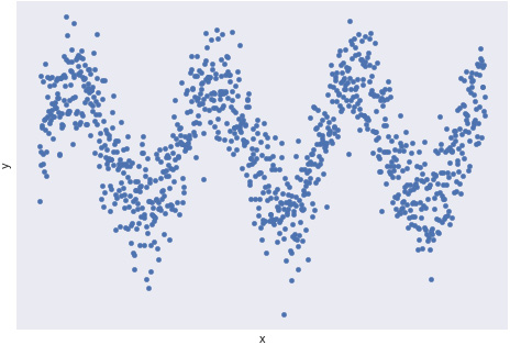
Another pattern people tend to look for is periodicity, that is, repeating patterns in the data. Such patterns can indicate that two variables may have cyclical behavior and can be useful in making predictions. The following diagram shows an example of periodic behavior:

Figure 1.19: An example of periodic behavior

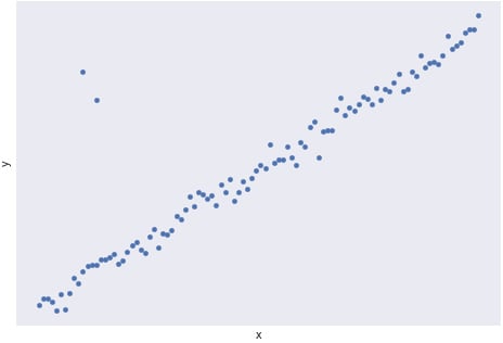
Another use of scatterplots is to help detect outliers. When most points in a graph appear to be in a specific region of the graph, but some points are quite far removed, this may indicate that those points are outliers with regard to the two variables. When performing further bivariate analysis, it may be wise to remove these points in order to reduce noise and produce better insights. The following diagram shows a case of points that may be considered outliers:

Figure 1.20: A scatterplot with two outliers

These techniques with scatterplots allow data professionals to understand the broader trends in their data and take the first steps to turn data into information.

Pearson Correlation Coefficient

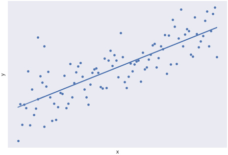
One of the most common trends in analyzing bivariate data is linear trends. Often times though, some linear trends are weak, while other linear trends are strong in how well a linear trend fits the data. In Figure 1.21 and Figure 1.22, we see examples of scatterplots with their line of best fit. This is a line calculated using a technique known as Ordinary Least Square (OLS) regression. Although OLS is beyond the scope of this book, understanding how well bivariate data fits a linear trend is an extraordinarily valuable tool for understanding the relationship between two variables:

Figure 1.21: A scatterplot with a strong linear trend

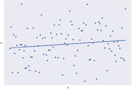
The following diagram shows a scatterplot with a weak linear trend:

Figure 1.22: A scatterplot with a weak linear trend

Note

For more information on OLS regression, please refer to a statistics textbook, such as Statistics by David Freedman, Robert Pisani, and Roger Purves.

One method for quantifying linear correlation is to use what is called the Pearson correlation coefficient. The Pearson correlation coefficient, often represented by the letter r, is a number ranging from -1 to 1, indicating how well a scatterplot fits a linear trend. To calculate the Pearson correlation coefficient, r, we use the following formula:

Figure 1.23: The formula for calculating the Pearson correlation coefficient

This formula is a bit heavy, so let's work through an example to turn the formula into specific steps.

Exercise 5: Calculating the Pearson Correlation Coefficient for Two Variables

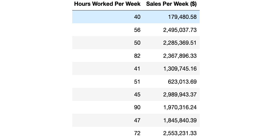
Let's calculate the Pearson correlation coefficient for the relationship between Hours Worked Per Week and Sales Per Week ($). In the following diagram, we have listed some data for 10 salesmen at a ZoomZoom dealership in Houston, and how much they netted in sales that week:

Figure 1.24: Data for 10 salesmen at a ZoomZoom dealership

Perform the following steps to complete the exercise:

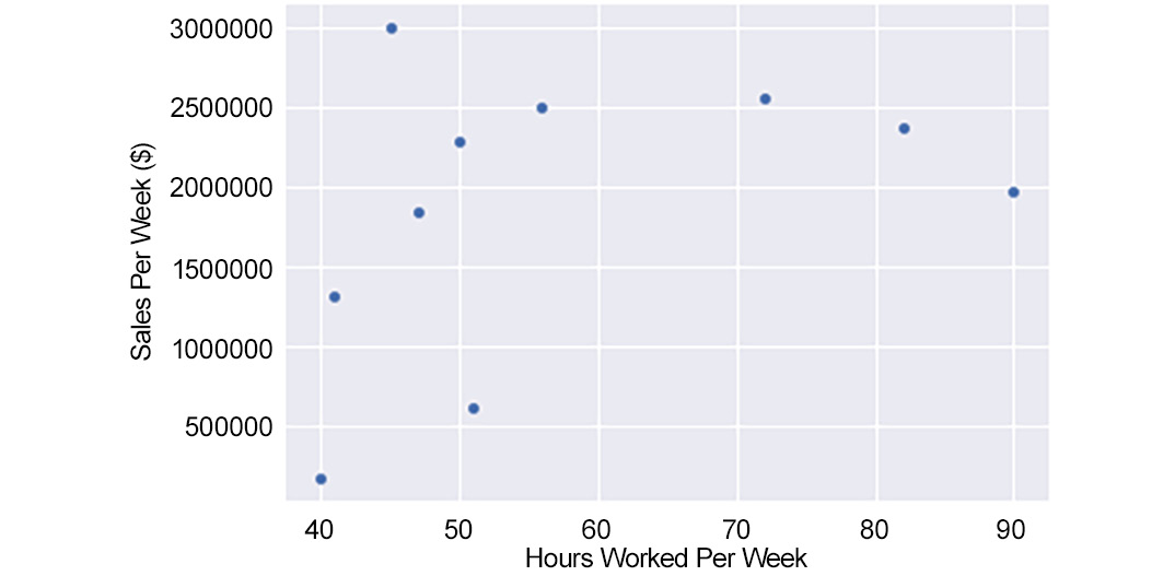
1. First, create a scatterplot of the two variables in Excel by using the data given in the scenario. This will help us to get a rough estimate of what to expect for the Pearson correlation coefficient:
   

   Figure 1.25: A scatterplot of Hours Worked Per Week and Sales Per Week

   There does not appear to be a strong linear relationship, but there does appear to be a general increase in Sales Per Week ($) versus Hours Worked Per Week.

2. Now, calculate the mean of each variable. You should get 57.40 for Hours Worked Per Week and 1,861,987.3 for Sales Per Week. If you are not sure how to calculate the mean, refer to the Central Tendency section.
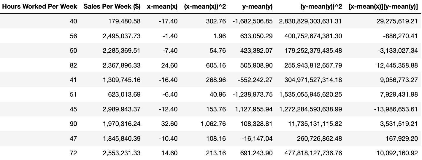
3. Now, for each row, calculate four values: the difference between each value and its mean, and the square of the difference between each value and its mean. Then, find the product of these differences. You should get a table of values, as shown in the following diagram:
   

   Figure 1.26: Calculations for the Pearson correlation coefficient

4. Find the sum of the squared terms and the sum of the product of the differences. You should get 2,812.40 for Hours Worked Per Week (x), 7,268,904,222,394.36 for Sales Per Week (y), and 54,492,841.32 for the product of the differences.
5. Take the square root of the sum of the differences to get 53.03 for Hours Worked Per Week (x) and 2,696,090.54 for Sales Per Week (y).
6. Input the values into the equation from Figure 1.27 to get 0.38. The following diagram shows the calculation:

Figure 1.27: The final calculation of the Pearson correlation coefficient

We learned how to calculate the Pearson correlation coefficient for two variables in this exercise and got the final output as 0.38 after using the formula.

Interpreting and Analyzing the Correlation Coefficient

Calculating the correlation coefficient by hand can be very complicated. It is generally preferable to calculate it on the computer. As you will learn in Chapter 3, SQL for Data Preparation, it is possible to calculate the Pearson correlation coefficient using SQL.

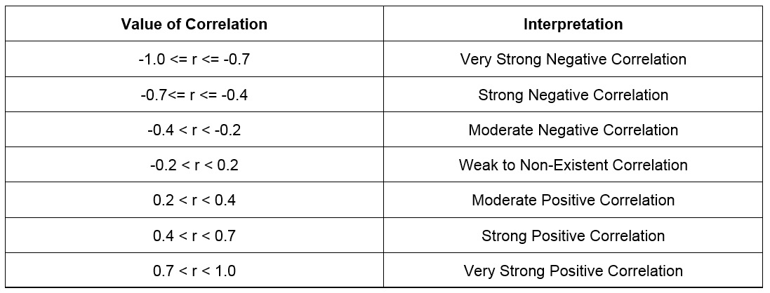
To interpret the Pearson correlation coefficient, compare its value to the table in Figure 1.28. The closer to 0 the coefficient is, the weaker the correlation. The higher the absolute value of a Pearson correlation coefficient, the more likely it is that the points will fit a straight line:

Figure 1.28: Interpreting a Pearson correlation coefficient

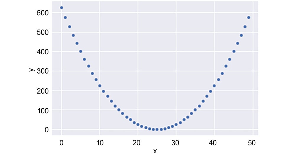
There are a couple of things to watch out for when examining the correlation coefficient. The first thing to watch out for is that the correlation coefficient measures how well two variables fit a linear trend. Two variables may share a strong trend but have a relatively low Pearson correlation coefficient. For example, look at the points in Figure 1.29. If you calculate the correlation coefficient for these two variables, you will find it is -0.08. However, the curve has a very clear quadratic relationship. Therefore, when you look at the correlation coefficients of bivariate data, be on the lookout for non-linear relationships that may describe the relationship between the two variables:

Figure 1.29: A strong non-linear relationship with a low correlation coefficient

Another point of importance is the number of points used to calculate a correlation. It only takes two points to define a perfectly straight line. Therefore, you may be able to calculate a high correlation coefficient when there are fewer points. However, this correlation coefficient may not hold when more data is presented into the bivariate data. As a rule of thumb, correlation coefficients calculated with fewer than 30 data points should be taken with a pinch of salt. Ideally, you should have as many good data points as you can in order to calculate the correlation.

Notice the use of the term "good data points." One of the recurring themes of this chapter has been the negative impact of outliers on various statistics. Indeed, with bivariate data, outliers can impact the correlation coefficient. Let's take a look at the graph in Figure 1.30. It has 11 points, one of which is an outlier. Due to that outlier, the Pearson correlation coefficient, r, for the data falls to 0.59, but without it, it equals 1.0. Therefore, care should be taken to remove outliers, especially from limited data:

Figure 1.30: Calculating r for a scatterplot with an outlier

Finally, one of the major problems associated with calculating correlation is the logical fallacy of correlation implying causation. That is, just because x and y have a strong correlation does not mean that x causes y. Let's take our example of the number of hours worked versus the number of sales netted per week. Imagine that, after adding more data points, it turns out that the correlation is 0.5 between these two variables. Many beginner data professionals and experienced executives would conclude that more working hours net more sales and start making their sales team work nonstop. While it is possible that working more hours causes more sales, a high correlation coefficient is not hard evidence for that. Another possibility may even be a reverse set of causation; it is possible that because you produce more sales, there is more paperwork and, therefore, you need to stay longer at the office in order to complete it. In this scenario, working more hours may not cause more sales. Another possibility is that there is a third item responsible for the association between the two variables.

For example, it may actually be that experienced salespeople work longer hours, and experienced salespeople also do a better job of selling. Therefore, the real cause is having employees with lots of sales experience, and the recommendation should be to hire more experienced sales professionals. As analytics professional, you will be responsible for avoiding pitfalls such as correlation and causation, and critically think about all the possibilities that might be responsible for the results you see.

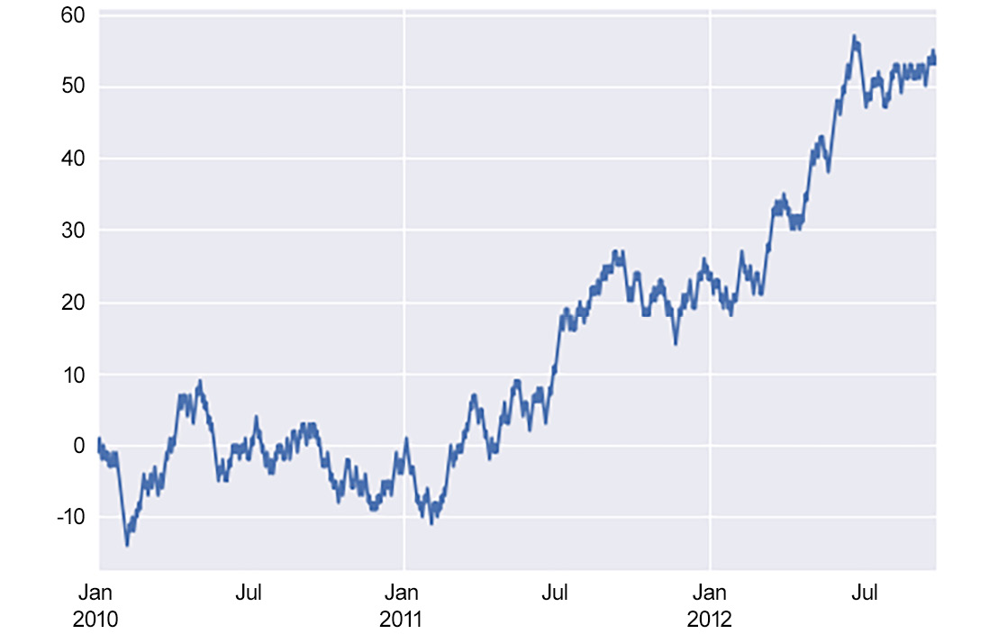
Time Series Data

One of the most important types of bivariate analysis is a time series. A time series is simply a bivariate relationship where the x-axis is time. An example of a time series can be found in Figure 1.31, which shows a time series from January 2010 to late 2012. While, at first glance, this may not seem to be the case, date and time information is quantitative in nature. Understanding how things change over time is one of the most important types of analysis done in organizations and provides a lot of information about the context of the business. All of the patterns discussed in the previous section can also be found in time series data. Time series are also important in organizations because they can be indicative of when specific changes happened. Such time points can be useful in determining what caused these changes:

Figure 1.31: An example of a time series

Activity 2: Exploring Dealership Sales Data

In this activity, we will explore a dataset in full. It's your first day at ZoomZoom, where the company is hard at work building the world's best electric vehicles and scooters in order to stop climate change. You have been recently hired as the newest senior data analyst for the company. You're incredibly excited to start your job and are ready to help however you can. Your manager, the head of analytics is happy to see you, but unfortunately, can't help you get set up today because of a company emergency (something about the CEO having a meltdown on a podcast). You don't have access to a database, but he did email you a CSV file with some data about national dealerships on it. He wants you to do some high-level analysis on annual sales at dealerships across the country:

1. Open the dealerships.csv document in a spreadsheet or text editor. This can be found in the Datasets folder of the GitHub repository.
2. Make a frequency distribution of the number of female employees at a dealership.
3. Determine the average and median annual sales for a dealership.
4. Determine the standard deviation of sales.
5. Do any of the dealerships seem like an outlier? Explain your reasoning.
6. Calculate the quantiles of the annual sales.
7. Calculate the correlation coefficient of annual sales to female employees and interpret the result.

   Note

   The solution for this activity can be found via this link.

Working with Missing Data

In all of our examples so far, our datasets have been very clean. However, real-world datasets are almost never this nice. One of the many problems you may have to deal with when working with datasets is missing values. We will discuss the specifics of preparing data further in Chapter 3, SQL for Data Preparation. Nonetheless, in this section, we would like to take some time to discuss some of the strategies you can use to handle missing data. Some of your options include the following:

• Deleting Rows: If a very small number of rows (that is, less than 5% of your dataset) are missing data, then the simplest solution may be to just delete the data points from your set. Such a result should not overly impact your results.
• Mean/Median/Mode Imputation: If 5% to 25% of your data for a variable is missing, another option is to take the mean, median, or mode of that column and fill in the blanks with that value. This may provide a small bias to your calculations, but it will allow you to complete more analysis without deleting valuable data.
• Regression Imputation: If possible, you may be able to build and use a model to impute missing values. This skill may be beyond the capability of most data analysts, but if you are working with a data scientist, this option could be viable.
• Deleting Variables: Ultimately, you cannot analyze data that does not exist. If you do not have a lot of data available, and a variable is missing most of its data, it may simply be better to remove that variable than to make too many assumptions and reach faulty conclusions.

You will also find that a decent portion of data analysis is more art than science. Working with missing data is one such area. With experience, you will find a combination of strategies that work well for different scenarios.

Another piece of analysis that is useful in data analysis is statistical significance testing. Often times, an analyst is interested in comparing the statistical properties of two groups, or perhaps just one group before and after a change. Of course, the difference between these two groups may just be due to chance.

An example of where this comes up is in marketing A/B tests. Companies will often test two different types of landing pages for a product and measure the click-through rate (CTR). You may find that the CTR for variation A of the landing page is 10%, and the CTR for variation B is 11%. So, does that mean that variation B is 10% better than A, or is this just a result of day-to-day variance? Statistical testing helps us to determine just that.

In statistical testing, there are a couple of major parts you need to have (Figure 1.32). First, we have the test statistic we are examining. It may be a proportion, an average, the difference between two groups, or a distribution. The next necessary part is a null hypothesis, which is the idea that the results observed are the product of chance. You will then need an alternative hypothesis, which is the idea that the results seen cannot be explained by chance alone. Finally, a test needs a significance level, which is the value the test statistic needs to take before it is decided that the null hypothesis cannot explain the difference. All statistical significance tests have these four aspects, and it is simply a matter of how these components are calculated that differentiate significance tests:

Figure 1.32: Parts of statistical significance testing

Common Statistical Significance Tests

Some common statistical significance tests include the following:

• Two-sample Z-test: A test to determine whether the averages of the two samples are different. This test assumes that both samples are drawn from a normal distribution with a known population standard deviation.
• Two-sample T-test: A test to determine whether the average of two samples is different when either the sample set is too small (that is, fewer than 30 data points per sample), or if the population standard deviation is unknown. The two samples are also generally drawn from distributions assumed to be normal.
• Pearson's Chi-Squared Test: A test to determine whether the distribution of data points to categories is different than what would be expected due to chance. This is the primary test for determining whether the proportions in tests, such as those in an A/B test, are beyond what would be expected from chance.

  Note

  To learn more about statistical significance, please refer to a statistics textbook, such as Statistics by David Freedman, Robert Pisani, and Roger Purves.

Data is a powerful method by which to understand the world. The ultimate goal for analytics is to turn data into information and knowledge. To accomplish this goal, statistics can be used to better understand data, especially descriptive statistics, and statistical significance testing.

One branch of descriptive statistics, univariate analysis, can be utilized to understand a single variable of data. Univariate analysis can be used to find the distribution of data by utilizing frequency distributions and quantiles. We can also find the central tendency of a variable by calculating the mean, median, and mode of data. It can also be used to find the dispersion of data using the range, standard deviation, and IQR. Univariate analysis can also be used to find outliers.

Bivariate analysis can also be used to understand the relationship between data. Using scatterplots, we can determine trends, changes in trends, periodic behavior, and anomalous points in regard to two variables. We can also use the Pearson correlation coefficient to measure the strength of a linear trend between the two variables. The Pearson correlation coefficient, however, is subject to scrutiny due to outliers or the number of data points used to calculate the coefficient. Additionally, just because two variables have a strong correlation coefficient does not mean that one variable causes the other variable.

Statistical significance testing can also provide important information about data. Statistical significance testing allows us to determine how likely certain outcomes are to occur by chance and can help us to understand whether the changes seen between groups are of consequence.

Now that we have the basic analytical tools necessary to understand data, we will now review SQL and how we can use it to manipulate a database in the next chapter.