Databricks provides a collaborative platform for data engineering and data science. Powered by the potential of Apache Spark™, Databricks helps enable ML at scale. It has also revolutionized the existing data lakes by introducing the Lakehouse architecture. You can refer to the following published whitepaper to learn about the Lakehouse architecture in detail: http://cidrdb.org/cidr2021/papers/cidr2021_paper17.pdf.
Irrespective of the data role in any industry, Databricks has something for everybody:
- Data engineer: Create ETL and ELT pipelines to run big data workloads.
- Data scientist: Perform exploratory data analysis and train ML models at scale.
- Data analyst: Perform big data analytics harnessing the power of Apache Spark.
- Business intelligence analyst: Build powerful dashboards using Databricks SQL Analytics.
Databricks and Spark together provide a unified platform for big data processing in the cloud. This is possible because Spark is a compute engine that remains decoupled from storage. Spark in Databricks combines ETL, ML, and real-time streaming with collaborative notebooks. Processing in Databricks can scale to petabytes of data and thousands of nodes in no time!
Spark can connect to any number of data sources, including Amazon S3, Azure Data Lake, HDFS, Kafka, and many more. As Databricks lives in the cloud, spinning up a Spark cluster is possible with the click of a button. We do not need to worry about setting up infrastructure to use Databricks. This enables us to focus on the data at hand and continue solving problems.
Currently, Databricks is available on all four major cloud platforms, Amazon Web Services (AWS), Microsoft Azure, Google Cloud Platform, and Alibaba Cloud. In this book, we will be working on Azure Databricks with the standard pricing tier. Databricks is a first-party service in Azure and is deeply integrated with the complete Azure ecosystem.
Since Azure Databricks is a cloud-native managed service, there is a cost associated with its usage. To view the Databricks pricing, check out https://azure.microsoft.com/en-in/pricing/details/databricks/.
Creating an Azure Databricks workspace
To create a Databricks instance in Azure, we will need an Azure subscription and a resource group. An Azure subscription is a gateway to Microsoft's cloud services. It entitles us to create and use Azure's services. A resource group in Azure is equivalent to a logical container that hosts the different services. To create an Azure Databricks instance, we need to complete the following steps:
- Go to Azure's website, portal.azure.com, and log in with your credentials.
- In the Navigate section, click on Resource groups and then Create.
- In Subscription, set the name of the Azure subscription, set a suitable name in Resource group, set Region, and click on Review + create.
- A Validation passed message will flash at the top; then, click on Create. Once the resource group is created, a notification will pop up saying Resource group created. Following the message, click on Go to resource group.
- This opens an empty resource group. Now it is time to create a Databricks instance. Click on Create and select Marketplace. In the search bar, type
Azure Databricks and select it from the drop-down menu. Click on Create.Figure 1.5 – Creating Azure Databricks
- Set Subscription, Resource group, a name, Region, and Pricing Tier (Standard, Premium, or Trial). In this book, we will be working with the standard pricing tier of Azure Databricks.
Figure 1.6 – Creating an Azure Databricks workspace
- Click on Next : Networking. We will not be creating Databricks in a VNet. So, keep both the options toggled to No. Finally, click on Review + create. Once the validation is successful, click on Create. It takes a few minutes for the Databricks instance to get created. Once the deployment is complete, click on Go to Resource. To launch the Databricks workspace, click on Launch Workspace.
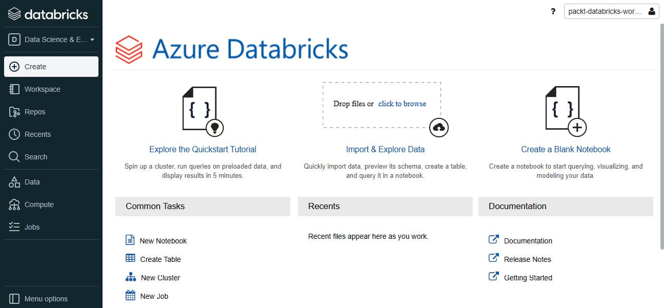
Figure 1.7 – Azure Databricks workspace
Now that we have a workspace up and running, let's explore how we can apply it to different concepts.
Core Databricks concepts
The Databricks workspace menu is displayed on the left pane. We can configure the menu based on our workloads, Data Science and Engineering or Machine Learning. Let's start with the former. We will learn more about the ML functionalities in Chapter 3, Learning about Machine Learning and Graph Processing with Databricks. The menu consists of the following:
- Workspace: A repository with a folder-like structure that contains all the Azure Databricks assets. These assets include the following:
- Notebooks: An interface that holds code, visualizations, and markdown text. Notebooks can also be imported and exported from the Databricks workspace.
- Library: A package of commands made available to a notebook or a Databricks job.
- Dashboard: A structured representation of the selective visualizations used in a notebook.
- Folder: A logical grouping of related assets in the workspace.
- Repos: This provides integration with Git providers such as GitHub, Bitbucket, GitLab, and Azure DevOps.
- Recents: Displays the most recently used notebooks in the Databricks workspace.
- Search: The search bar helps us to find assets in the workspace.
- Data: This is the data management tab that is built on top of a Hive metastore. Here, we can find all the Hive tables registered in the workspace. The Hive metastore stores all the metadata information, such as column details, storage path, and partitions, but not the actual data that resides in a cloud storage location. The tables are queried using Apache Spark APIs including Python, Scala, R, and SQL. Like any data warehouse, we need to create a database and then register the Hive tables.
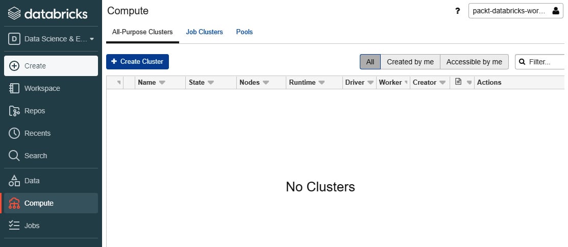
- Compute: This is where we interact with the Spark cluster. It is further divided into three categories:
- All-Purpose Clusters: These are used to run Databricks notebooks and jobs. An all-purpose cluster can also be shared among users in the workspace. You can manually terminate or restart an all-purpose cluster.
- Job Clusters: These are created by the Azure Databricks job scheduler when a new job is created. Once the job is complete, it is automatically terminated. It is not possible to restart a job cluster.
- Pools: A pool is a set of idle node instances that help reduce cluster start up and autoscaling times. When a cluster is attached to a pool, it acquires the driver and worker instances from within the pool.
Figure 1.8 – Clusters in Azure Databricks
- Jobs: A job is a mechanism that helps to schedule notebooks for creating data pipelines.
Now that we have an understanding of the core concepts of Databricks, let's create our first Spark cluster!
Creating a Spark cluster
It is time to create our first cluster! In the following steps, we will create an all-purpose cluster and later attach it to a notebook. We will be discussing cluster configurations in detail in Chapter 4, Managing Spark Clusters:
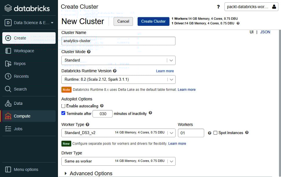
- Select the Clusters tab and click on Create Cluster. Give an appropriate name to the cluster.
- Set Cluster Mode to Standard. Standard cluster mode is ideal when there is a single user for the cluster. High Concurrency mode is recommended for concurrent users, but it does not support Scala. A Single Node cluster has no worker nodes and is only suitable for small data volumes.
- Leave the Pool option as None and Databricks Runtime Version as the default value. The Databricks runtime version decides the Spark version and configurations for the cluster.
- For Autopilot Options, disable the Enable autoscaling checkbox. Autoscaling helps the cluster to automatically scale between the maximum and minimum number of worker nodes. In the second autopilot option, replace 120 with 030 to terminate the cluster after 30 minutes of inactivity.
- We can leave the Worker Type and Driver Type options as their default values. Set the number of workers to
01. Keep the Spot instances checkbox disabled. When enabled, the cluster uses Azure Spot VMs to save costs.
- Click on Create Cluster.
Figure 1.9 – Initializing a Databricks cluster
With the Spark cluster initialized, let's create our first Databricks notebook!
Databricks notebooks
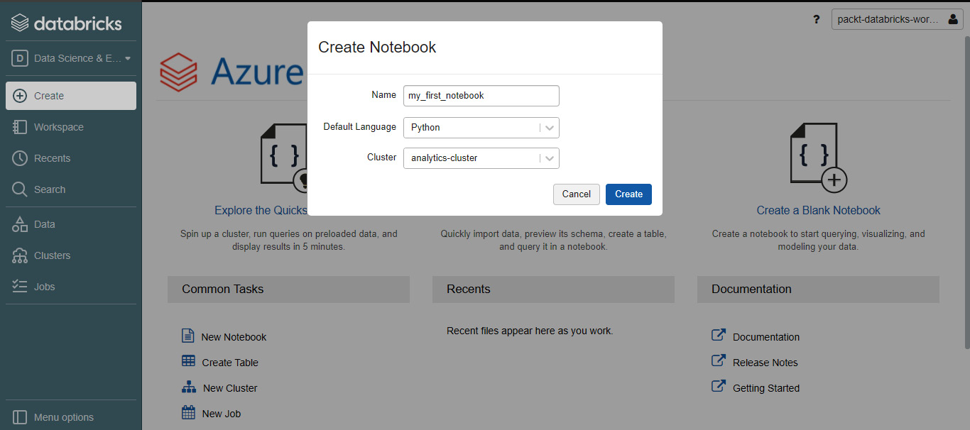
Now we'll create our first Databricks notebook. On the left pane menu, click on Create and select Notebook. Give a suitable name to the notebook, keep the Default Language option as Python, set Cluster, and click on Create.
Figure 1.10 – Creating a Databricks notebook
We can create documentation cells to independently run blocks of code. A new cell can be created with the click of a button. For people who have worked with Jupyter Notebooks, this interface might look familiar.
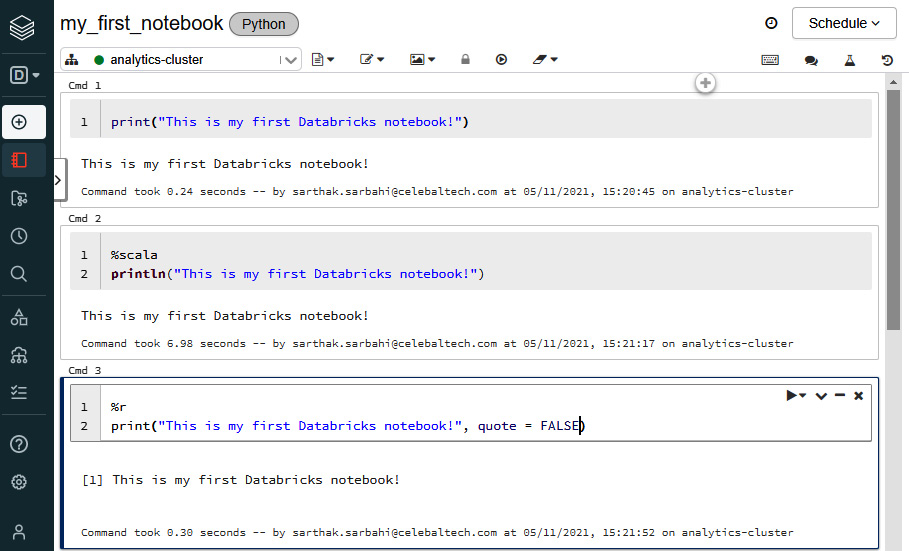
We can also execute code in different languages right inside one notebook. For example, the first notebook that we've created has a default language of Python, but we can also run code in Scala, SQL, and R in the same notebook! This is made possible with the help of magic commands. We need to specify the magic command at the beginning of a new cell:
Let us look at executing code in multiple languages in the following image:
Figure 1.11 – Executing code in multiple languages
We can also render a cell as Markdown using the %md magic command. This allows us to add rendered text between cells of code.
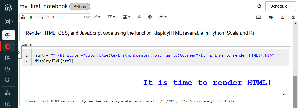
Databricks notebooks also support rendering HTML graphics using the displayHTML function. Currently, this feature is only supported for Python, R, and Scala notebooks. To use the function, we need to pass in HTML, CSS, or JavaScript code:
Figure 1.12 – Rendering HTML in a notebook
We can use the %sh magic command to run shell commands on the driver node.
Databricks provides a Databricks Utilities (dbutils) module to perform tasks collectively. With dbutils, we can work with external storage, parametrize notebooks, and handle secrets. To list the available functionalities of dbutils, we can run dbutils.help() in a Python or Scala notebook.
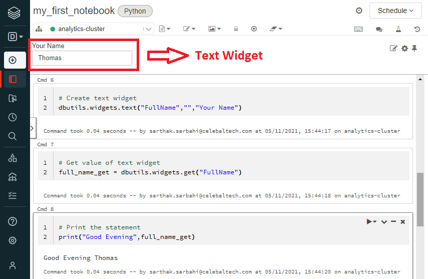
The notebooks consist of another feature called widgets. These widgets help to add parameters to a notebook and are made available with the dbutils module. By default, widgets are visible at the top of a notebook and are categorized as follows:
- Text: Input the string value in a textbox.
- Dropdown: Select a value from a list.
- Combobox: Combination of text and drop-down widgets.
- Multiselect: Select one or more values from a list:
Figure 1.13 – Notebook widget example. Here, we create a text widget, fetch its value, and call it in a print statement
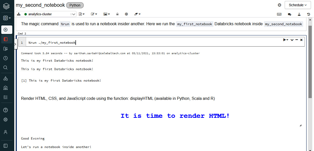
We can also run one notebook inside another using the %run magic command. The magic command must be followed by the notebook path.
Figure 1.14 – Using the %run magic command
Databricks File System (DBFS)
DBFS is a filesystem mounted in every Databricks workspace for temporary storage. It is an abstraction on top of a scalable object store in the cloud. For instance, in the case of Azure Databricks, the DBFS is built on top of Azure Blob Storage. But this is managed for us, so we needn't worry too much about how and where the DBFS is actually located. All we need to understand is how can we use DBFS inside a Databricks workspace.
DBFS helps us in the following ways:
- We can persist data to DBFS so that it is not lost after the termination of the cluster.
- DBFS allows us to mount object storage such as Azure Data Lake or Azure Blob Storage in the workspace. This makes it easy to access data without requiring credentials every time.
- We can access and interact with the data using the directory semantics instead of using URLs for object storage.
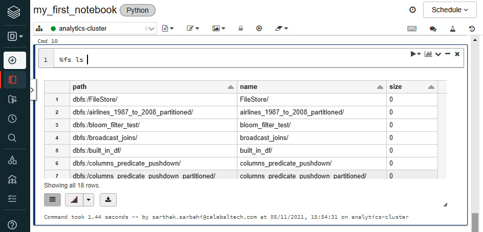
DBFS has a default storage location called the DBFS root. We can access DBFS in several ways:
- With the
%fs magic command: We can use the %fs command in a notebook cell.
- With
dbutils: We can call the dbutils module to access the DBFS. Using dbutils.fs.ls("<path>") is equivalent to running %fs ls <path>. Here, <path> is a DBFS path. Both these commands list the directories in a specific DBFS "path."
Figure 1.15 – Listing all files in the DBFS root using the %fs magic command
Note
We need to enclose dbutils.fs.ls("path") in Databricks' display() function to obtain a rendered output.
Databricks jobs
A Databricks job helps to run and automate activities such as an ETL job or a data analytics task. A job can be executed either immediately or on a scheduled basis. A job can be created by using the UI or CLI or invoking the Jobs UI. We will now create a job using the Databricks UI:
- Create a new Databricks Python notebook with the name
jobs-notebook and paste the following code in a new cell. This code creates a new delta table and inserts records into the table. We'll learn about Delta Lake in more detail later in this chapter. Note that the following two code blocks must be run in the same cell.The following code block creates a delta table in Databricks with the name of insurance_claims. The table has four columns, user_id, city, country, and amount:
%sql
-- Creating a delta table and storing data in DBFS
-- Our table's name is 'insurance_claims' and has four columns
CREATE OR REPLACE TABLE insurance_claims (
  user_id INT NOT NULL,
  city STRING NOT NULL,
  country STRING NOT NULL,
  amount INT NOT NULL
)
USING DELTA
LOCATION 'dbfs:/tmp/insurance_claims';
Now, we will insert five records into the table. In the following code block, every INSERT INTO statement inserts one new record into the delta table:
INSERT INTO insurance_claims (user_id, city, country, amount)
VALUES (100, 'Mumbai', 'India', 200000);
INSERT INTO insurance_claims (user_id, city, country, amount)
VALUES (101, 'Delhi', 'India', 400000);
INSERT INTO insurance_claims (user_id, city, country, amount)
VALUES (102, 'Chennai', 'India', 100000);
INSERT INTO insurance_claims (user_id, city, country, amount)
VALUES (103, 'Bengaluru', 'India', 700000);
- On the workspace menu, click on Jobs and then Create Job. Give a name to the job and keep Schedule Type as Manual (Paused). Under the Task heading, set Type to Notebook, select the
jobs-notebook notebook that we created, and in Cluster, select an existing all-purpose cluster.
- Keep Maximum Concurrent Runs at the default value of 1. Under Alerts, click on Add. Add the email address to which alerts must be sent and select Success and Failure. This will ensure that the designated email address will be notified upon a job success or failure.
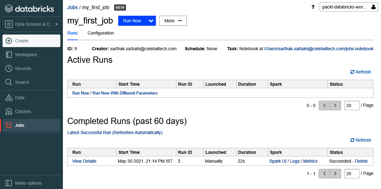
- Click on Create. Once the job is created, click on Runs and select Run Now.
- As soon as the job completes, we will receive an email informing us whether the job succeeded or failed. If the job is in progress, we can find more information about the current run under Active Runs.
- When the job finishes, a new record will be added under Completed Runs (past 60 days) giving the start time, mode of launch, duration of run, and status of run.
Figure 1.16 – Successful manual run of a Databricks job
Databricks Community
Databricks Community is a platform that provides a free-of-cost Databricks workspace. It supports a single node cluster wherein we have one driver and no workers. The community platform is great for beginners to get started with Databricks. But several features of Azure Databricks are not supported in the Community edition. For example, we cannot create jobs or change cluster configuration settings. To sign up for Databricks Community, visit https://community.cloud.databricks.com/login.html.
 Argentina
 Australia
 Austria
 Belgium
 Brazil
 Bulgaria
 Canada
 Chile
Chile
 Colombia
 Cyprus
 Czechia
 Denmark
 Ecuador
 Egypt
Egypt
 Estonia
 Finland
 France
 Germany
 Great Britain
 Greece
 Hungary
 India
India
 Indonesia
 Ireland
 Italy
Italy
 Japan
Japan
 Latvia
 Lithuania
 Luxembourg
 Malaysia
 Malta
Malta
 Mexico
 Netherlands
 New Zealand
 Norway
 Philippines
 Poland
 Portugal
 Romania
 Russia
 Singapore
 Slovakia
 Slovenia
 South Africa
 South Korea
 Spain
Spain
 Sweden
 Switzerland
 Taiwan
 Thailand
 Turkey
 Ukraine
 United States